
- Submit a Protocol
- Receive Our Alerts
- EN

- Protocols

- Articles and Issues
- For Authors
- About
- Become a Reviewer

Studying Chemotactic Migration in Dunn Chamber: An Example Applied to Adherent Cancer Cells
Published: Vol 12, Iss 3, Feb 5, 2022 DOI: 10.21769/BioProtoc.4316 Views: 1662
Reviewed by: Alak MannaBeom K ChoiAnonymous reviewer(s)
Original research article
The authors used this protocol in:

Jan 2013

Protocol Collections
Comprehensive collections of detailed, peer-reviewed protocols focusing on specific topics


Abstract
Cell migration is a vital process in the development of multicellular organisms. When deregulated, it is involved in many diseases such as inflammation and cancer metastisation. Some cancer cells could be stimulated using chemoattractant molecules, such as growth factor Heregulin β1. They respond to the attractant or repellent gradients through a process known as chemotaxis. Indeed, chemotactic cell motility is crucial in tumour cell dissemination and invasion of distant organs. Due to the complexity of this phenomenon, the majority of available in vitro methods to study the chemotactic motility process have limitations and are mainly based on endpoint assays, such as the Boyden chamber assay. Nevertheless, in vitro time-lapse microscopy represents an interesting opportunity to study cell motility in a chemoattracting gradient, since it generates large volume image-based information, allowing the analysis of cancer cell behaviours. Here, we describe a detailed time-lapse imaging protocol, designed for tracking T47D human breast cancer cell line motility, toward a gradient of Heregulin β1 in a Dunn chemotaxis chamber assay. The protocol described here is readily adapted to study the motility of any adherent cell line, under various conditions of chemoattractant gradients and of pharmacological drug treatments. Moreover, this protocol could be suitable to study changes in cell morphology, and in cell polarity.
Background
Directed migration is a key process implicated in physiological and in pathological phenomena, like wound-healing and metastasis. When a cell polarizes and migrates in a directed way, in response to a ligand simulation, it is called chemotactic migration (Stuelten et al., 2018). In adherent and non-adherent cells, migration engages cytoskeletal components and regulators in different manners; chemotactic migration involves close but dissimilar mechanisms, depending on cell types and experimental conditions (Entschladen et al., 2005). To analyse chemotactic migration, various devices have been generated, among which is the classical Boyden chamber assay (transwell assay). In the Boyden chamber assay, cells migrate from the upper to the lower side of a porous membrane, through a gradient of chemoattractant. This assay is valuable for adherent and non-adherent cells, and it offers 3D migration conditions. But its major limitation is that cells can’t be studied while migrating, as with live-cell microscopy. The end results of chemotactic migration in the Boyden chamber are deduced after cell fixation and staining (Chen, 2012). With the development of time-lapse microscopy, based on phase contrast that causes less photodamage, experiments of live-cell imaging for longer periods have become easier to perform. Thus, many 2D random migration devices (Gau and Roy, 2020), and 2D chemotaxis migration devices have been generated (Taylor et al., 2018), such as the ibidi μ-Slide Chemotaxis® (Zengel et al., 2011). One of the first, and efficient 2D chemotaxis migration assays is the Dunn chemotaxis chamber assay (Zicha et al., 1991). It is a glass chamber, with an inner well free of chemoattractant, and an outer well that contains chemoattractant. Hence, a gradient of chemoattractant is formed on the annular bridge between the two wells. Cells are directly observed while migrating on this bridge, using a time-lapse microscope. A detailed description of the assay is available elsewhere (Monypenny et al., 2009; Chaubey et al., 2011).
Dunn chamber assembly is a multistep process that requires good manual dexterity (Taylor et al., 2018). This might be the reason why it is not frequently used. In this protocol, we will explain how to use the Dunn chamber and how to analyse its results, step by step. The essential contribution of this protocol is that we tried to simplify some steps, in assembly and in analysis, and make them user-friendly, to facilitate the use this device. Finally, we used T47D cells in this protocol (Benseddik et al., 2013). However, any adherent cell line could be used with its respective chemoattractant. Plus, cell morphology and polarity could also be closely observed and analysed within this assay.
Materials and Reagents
Hard non curling glass coverslips, No. 3 or No. 2 (Ted Pella, catalog number: 260156)
35 mm culture dishes (Corning, Costar, catalog number: CLS430588)
15 mL conical centrifuge tubes (BD, catalog number: 14-959-49D)
Sterile filter paper (Thermo Fisher Scientific, catalog number: 09-802-1B)
2.5 cm conventional injection needle (Thermo Fisher Scientific, catalog number: 14-817-144)
T47D human breast carcinoma cells (ATCC®, number HTB-133TM)
Dulbecco's modified eagle medium DMEM (Lonza, BioWhittaker, catalog number: BW12-604F)
Heat-inactivated FBS (Corning, catalog number: 35011CV)
100× Antibiotic Penicillin-Streptomycin (Gibco, catalog number: 15140148) (to prevent bacterial and fungal contamination of cell culture)
100× Sodium pyruvate (Gibco, catalog number: 11360-070)
Collagen I, 3 mg/mL (Gibco, catalog number: A1048301)
Phosphate buffered saline (PBS) (Lonza, BioWhittaker, catalog number: BW17516F)
Trypsin-EDTA (Lonza, Trypsin-Versene, catalog number: BW17161E)
Heregulin β1 (HRGβ1) (R&D Systems, catalog number: 396-HB)
Trypan Blue Solution 0.4% (Gibco, catalog number: 15250061)
Dunn chamber (Hawksley, catalog number: DCC100)
DMEM S+ media (see Recipes)
Collagen solution (10 μg/mL) (see Recipes)
Equipment
Flat tweezer (Thermo Fisher Scientific, catalog number: 12342158)
Cell culture incubator set to 37°C and 5% CO2 (Thermo Fisher Scientific, catalog number: 51030303)
Waterbath set to 37°C (Thermo Fisher Scientific, catalog number: TSCIR35)
Class II Type A2 Biological Safety Cabinet (cell culture hood)
Counting chamber Malassez (Marienfeld Superior, catalog number: 0640610)
Motorized Inverted microscope Axiovert 200 M (Carl Zeiss)
Live-cell imaging environmental chamber with 5% (v/v) CO2 in air at 37°C (Climabox, Carl Zeiss)
Camera for microscope (Coolsnap HQ; Roper Scientific®)
10× objective [10× plan apochromat (NA 1.4) objective; Carl Zeiss]
Software
MetaMorph Microscopy Automation and Image Analysis Software® (Molecular Devices)
Chemotaxis and migration tool 1.01, ImageJ Plugin® (ibidi)
ImageJ® (National Institutes of Health)
Microsoft Excel (Microsoft®)
Procedure
Collagen I coating
Place a sterilised coverslip into each culture dish.
Coat coverslips with 500 μL of Collagen-I solution (composition described below) for 1 h at 37°C, then wash gently with 2 mL of PBS.
Immediately put 2 mL of DMEM S+ media (composition described below) in culture dishes, to prevent drying.
Cell culture
Use Human T47D cells at 70% confluency.
Culture cells in DMEM S+ media.
Wash cells twice with 1× PBS then add 1 mL of Trypsin. Incubate 5 min at 37°C.
Add 2 mL of DMEM S+ media to inactivate Trypsin.
Break down into individual cells by pipetting up and down gently, and then place them in 15 mL conical centrifuge tubes.
Spin the cells down by centrifuging 3 min at 300× g.
Aspirate supernatant and resuspend cells in 2 mL of DMEM S+ media.
Mix 100 µL of cell suspension with an equal volume of Trypan Blue Solution, and count cells using Malassez counting cell.
Put 105 resuspended cells in each well (when needed, cells may be transfected with a siRNA or a plasmid, before spreading).
Incubate cells in cell culture incubator for two days, for optimal adherence and migration.
Dunn migration assay
Prewarm sterile Dunn chambers in cell culture incubator for 30 min [Dunn chamber is described at Chaubey et al. (2011) and Monypenny et al. (2009)].
Warm-up DMEM S+ media in water bath.
Put enough DMEM S+ media to cover the whole chamber, with the two wells and the bridge, forming a round-shaped drop.
Change the media, to remove any dead cells, then pick the coverslip out of the well using the sterile injection needle and grip it with the flat tweezers.
Invert the coverslip and lower it on the Dunn chamber, so that the seeded area is aligned with the wells. Leave a very tight opening (0.5 mm).
Press gently but tightly on the outer edges of the coverslip, using sterile filter paper. Once the coverslip is dry, a barrier is created by media surface tension. At this stage, you should see Newton rings. Consequently, the coverslip strongly adheres to the chamber, during hours, with no air or media leakage.
Empty the outer well through the tight opening using sterile filter paper. The media will be slowly drawn by capillarity.
Fill the empty outer well with DMEM S+ media supplied with HRGβ1 at 10 nM.
Cautiously push the coverslip 2-3 mm, just enough to seal the tight opening. The gradient will be stable for at least 8 h (Benseddik et al., 2013).
See Note 1 for more information.
Cell imaging
Previously warm up the live-cell imaging microscope and its live-cell imaging environmental chamber for 1 h to equilibrate the temperature.
Place the Dunn chamber on the stage and fix it with clips, then place it on the specimen chamber, and equilibrate the temperature for 15 min.
Select fields with the annular bridge, with no more than seven single cells. Always include the outer border of the bridge in the microscope field, to identify the gradient direction.
Use Metamorph® software or any cell tracking software for time lapse image acquisition, and set time-lapse imaging for 4 h with 1 frame each 4 min, using phase-contrast. Note that the frames and the total duration are set according to the speed (velocity) of each cell type.
Save files and start time-lapse imaging. At the end of imaging, each field is saved in an individual folder that contains one image stack.
See Note 2 for more information.
Data analysis
Metamorph® analysis
Open one image stack in Metamorph® software.
If you could not rotate the camera during image acquisition, then rotate the image stacks using the “Rotate” command in the “Display” Menu, so that the outer border of the bridge becomes oriented to the top of the monitor screen. Consequently, image stack rotation allows the HRGβ1 gradient direction, oriented from the inner well to the outer well, to become vertically reoriented from bottom to top. Thus, the HRGβ1 gradient axis is aligned to y-axes during cell tracking (Figure 1).
Save the specific rotation angle value (θ) of each image stack (each field). After tracking, the rotation angle value of each field will be used to readjust all x and y coordinates (see below).
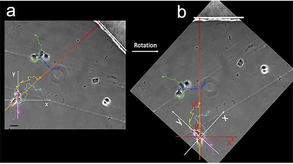
Figure 1. An example of image rotation and deviation angle measurement. Cell trajectories are labelled in cyan, yellow, pink, green, or blue. Scale bar, 20 µm. (a). A straight line (white) tangential to the outer border of the bridge is perpendicular to the bottom-up oriented HRGβ1 gradient axis (orange-red). As previously explained, when you set the track origin options of each cell at “first point in track”, x and y axes for each cell are parallel to monitor screen edges (white coordinate plane). (b). To correctly analyse cell behaviour, and adjust trajectory coordinates according to the HRGβ1 gradient direction, you should overlap the y-axis (red coordinate plane) on the gradient axis (orange-red). Rotate the image stack until the outer limit of the bridge gets up into the top. The rotation angle corresponds to the deviation angle (θ) of the y axis from the gradient axis. Note that the same deviation angle is accepted for cells sharing the same field (e.g., cells with cyan, yellow, or pink trajectories). In this example, the deviation angle is 45°.To track cells, open “Track objects” in “apps”.
Select the frames (planes) you want to analyse in your image stack.
Open Microsoft Excel® and pick the required measurements at “Config Log”. Then click on “Log Data” (Figure 2, step 1).
Set “Search Options”: At “Algorithm”, select “Template Match”. At “Delay”, choose a reasonable delay so you can easily observe cells (0.4 s/object). After that, check “Update Template Each Frame” and “Use derivative image”, then click “OK” (Figure 2, step 2).
Set the “Track Objects Interval Options”: For T47D cells, it was one image capture every 4 min (Figure 2, step 3).
Set the “Track Overlay Options”: check “Display point on current plane” and “Highlight display track path “. You can adjust at your convenience the colour and type of the track point (Figure 2, step 4).
Set “Origin Options” at “First point in track” (Figure 2, step 5): Axes origin coordinates (0, 0) correspond to each cell position in the first frame, x and y axes are parallel to monitor screen edges.
Track cells whose trajectories are not blocked by any obstacles.
Click on “Track”, precise sizes of objects, and sizes of regions in which the software should search for the cell (Figure 2, step 6 and step 7). Sizes depend on cell size and cell speed. In our experiments, object size was defined by cell nucleus, as it does not change shape during migration.
To select a cell, click on it with key “Control” pressed down. Once you have selected all cells you want to track, click “OK” to begin tracking.
Metamorph® allows you to track cells automatically. But if an error appears in your monitor screen, you can stop tracking using the key “Escape”, and click on “Step Back”, correct the position, then click “Update Position And Continue” (Figure 2, step 8).
When all the selected frames are analysed, tracking stops spontaneously. The tracking information you need is generated in an Excel file, on “Display Statistic” (Figure 2, step 9). For ImageJ analysis, you need (x, y) coordinates.
Repeat those steps for all images stacks. An image example after rotation and tracking is available in Figure 1.
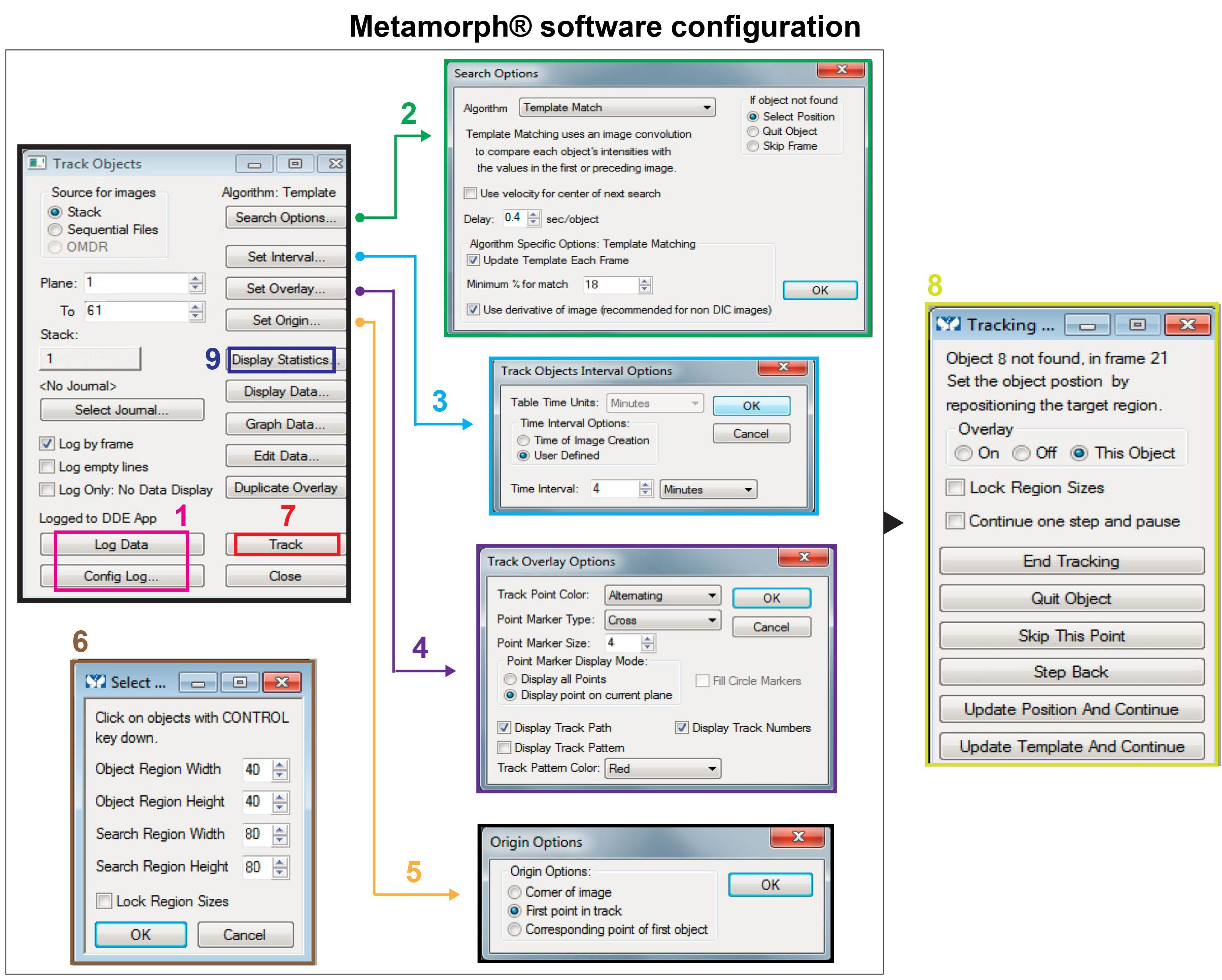
Figure 2. A plan summing up the essential settings required for cell tacking on Metamorph® software. The detailed settings of the menu options numbered from 1 to 9 are listed in the above text.
Preparing a file for ImageJ analysis
Open the Excel file of each image stack. The spreadsheet must contain essentially the x, y position coordinates per frame, plus other information according to your adjustments on Metamorph® “Display Statistic”.
Remember, since the Dunn chamber has an annular form, in most of the observed fields the y-axis of tracked cells are not aligned with the HRGβ1 gradient axis. Thus, you have previously performed image stacks rotations, so that y-axes become parallel to the gradient axis. Each field has a rotation angle (θ) you have saved during the analysis step on Metamorph®.
See Note 3 for more information.
Adjust all x, y position coordinates using the rotation angle (θ). To rotate (x, y) around the origin (0, 0) by θ degree, simply apply this Theorem (θ is in radian):
𝑥’= 𝑥cos θ − ysin θ
𝑦’= 𝑥sin θ + ycos θSave new (x’, y’) position coordinates in the same spreadsheet with other migration parameters information (Figure 3). Those new (x’, y’) position coordinates correspond to the final (x, y) coordinates you will use in ImageJ analysis.
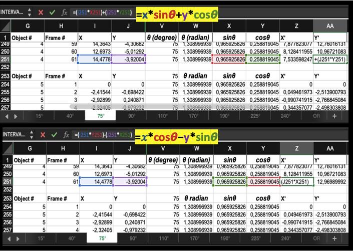
Figure 3. An example of data analysis and x, y coordinate rotation using the mathematic formula on Excel. Cell tracking information of the same image stack is gathered in one spreadsheet. Here, we assembled all spreadsheets of a single experiment in one Excel file. In this example of a spreadsheet, column G contains object (cell) number, column H contains frame number, and columns I and J contain (x, y) coordinates of each frame. All additional information, about the rotation angle θ and the (x’, y’) new coordinates, are added manually on the Excel spreadsheet. In this example, the rotation angle is 75°, it is added in column V. Columns W, X, and Y contain calculations that we use for the rotation formula, to readjust coordinates (x, y) to (x’, y’). The formula for y’ coordinates are in column Z, highlighted in the upper screenshot. The formula for x’ coordinates are in column AA, highlighted in the lower screenshot.In a new Excel file, gather information for different cells in a single experiment, or a group of similar experiments one after another, in the same spreadsheet (Figure 4):
The file must be organized in this order: Image plane, Object, frame, x' coordinate, y' coordinate.
If a comma was previously used as a decimal point, replace all commas with points.
The first Excel cell must contain writing regardless of the characters, and there must be no space between lines or columns. Supplementary information or spreadsheets must be removed.
First save it to a “.xls” file to keep its properties, then save a second file as “.txt” (Text (Tab delimited)) to use it for ImageJ analyses.
See Note 4 for more information.
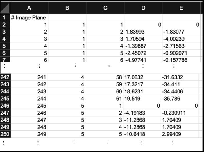
Figure 4. An example of Excel file as prepared for analysing on Chemotaxis and Migration Tool 1.01. The file contains one spreadsheet with: writing in A1 cell, then in second line Image plane number, Object number, frame number, and finally x' coordinate and y' coordinate.
ImageJ analyses
Install the plugin “Chemotaxis and Migration Tool” Version 1.01 in ImageJ, and open it.
At “Import data”, add the “.txt” file you want to analyse.
Set “number of slices”: Put the number of frames specific to your experiment. In our case it was 61 frames.
At “Settings”, add the unit (µm), and the time interval that corresponds to time-lapse imaging frequency. In our experiment, it was a frame every 4 min.
Now, back to "Import dataset”, click on “Add dataset”. Then, choose “Selected Dataset 1”, and finally click on “Apply settings”.
Summed up information about migration parameters are available by clicking at “Show info”.
At “Plot feature” tab, choose “Mark up/down” at “Set marking”, choose also “Open in new window”, “Show centre of mass”, and “Show additional info”.
Display vector plot by clicking on “Plot graph”, and use the default graphical settings (labels, axes, range, etc.), or adjust them by clicking on “more >>” at the bottom of the plot (Figure 5).
Under "Diagram feature" tab, choose “Open in new window” and “Show additional info”, The “Interior angle” and the “Range interval” are automatically adjusted at 66° and 10°, respectively.
Click on “Plot Rose diagram” to display a rose diagram plot, and use the default graphical settings (labels, axes, range, etc.), or adjust them by clicking on “more >>”, at the bottom of the rose plot (Figure 4).
Under “Statistic feature” tab, click on “Series function” in the scrolling menu, to get supplementary details about migration and chemotaxis parameters: Velocity, Distance, Directionality (directional persistence), Forward migration index, Centre of mass, etc.
To explore directional response to the gradient, perform Rayleigh test. Click on “Rayleigh test” on the scrolling menu. In “Distance from origin” choose “Use endpoints”, then click on “Compute Rayleigh Test”. The Rayleigh test verifies cell scattering using endpoints x, y coordinates:
When P > 0.05, this means cell scattering is homogenous, thus cells show no preference in directionality while they are migrating.
When P < 0.05, this means that cell scattering is oriented in a given direction.
To further confirm that cells are showing a significant response up the gradient of HRGβ1, you may calculate the confidence interval. The confidence interval for the mean cell direction (centre of mass of all endpoints) must be in the same direction as the HRGβ1 gradient. To calculate the confidence interval:
Go to “Series function” in scrolling menu under “Statistic feature” tab. Get x, y endpoints values by clicking on “Directionality”.
Copy the whole table in a new Excel spreadsheet, then use endpoints x, y coordinates to calculate the confidence interval (alpha = 0.05).
You may draw the two arrows that represent minimum and maximum values of calculated confidence interval on the vector plot. If there is a directional response to the gradient, the sector formed by these arrows should be in the same direction as the HRGβ1 gradient (Figure 5).
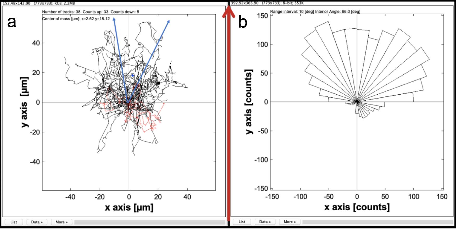
Figure 5. Examples of plots that represent chemotaxis migration. The red arrow indicates the HRGβ1 gradient axis. (a). A vector plot showing individual cell trajectories. Cells whose final positions are in the lower part of the graph are in red, and cells in the upper part of the graph are in black. Centre of mass (blue point) and confidence interval (blue arrows) are drawn to statistically represent chemotaxis migration in the plot. (b). A rose plot (also called circular histogram) shows the chemotactic tendency of whole cells. Each segment (10°) area represents a count of cells whose positions fit in the chosen angle (interior angle 66°).See Note 5 for more information.
Notes
The last steps in Dunn chamber assembly must be conducted extremely carefully. Please note that:
If the coverslip is uncarefully stirred, this can crush the cells.
In case the coverslip is not thick enough, then its flexibility will disturb chemoattractant gradient.
Do not over-drain the outer well.
Filling the outer well must be done passively with no pressure. A racked micropipette tip that fits is placed on the tight opening, and the media is “poured” gently.
A hot sealing mixture is used by Zicha et al. (1991) to seal the opening. However, using a dye to fill the outer well, we verified the possibility to seal the opening with no disturbance of the gradient, just by gently pushing the coverslip 2 mm. This result was then confirmed using HRGβ1, with directed migration of T47D cells. To appropriately perform this gesture, it is recommended to do some practising with a dye.
Air bubbles should absolutely be avoided because they cause distortion in the gradient. Do not hesitate to prepare multiple devices in parallel for each experimental condition, to be sure of ending with at least one without air bubbles.
While manipulating, transporting, or installing the Dunn chamber for live-cell imaging, never press on or shake it.
Given the thickness of the coverslip, it is not possible to use high magnification. Hence, it is not possible to analyse subcellular structures using the Dunn chamber.
If possible, rotate the camera to align the outer border of the bridge to the top of the monitor screen, which will facilitate the mathematical analysis of your data. This was not possible with our camera.
Image stacks were rotated, in order to align y axes of tracked cells on the HRGβ1 gradient axis. However, Metamorph® software does not take these rotations into account for cell tracking, and (x, y) position coordinates are still established according to the original coordinate plane (before video rotation). Still, this rotation allows precise estimation of the deviation angle “θ” of y-axis from the gradient axis (θ) (Figure 1). θ angle is then used in mathematical calculations to adjust coordinates (Figure 3).
Before analysing your data on Chemotaxis and Migration Tool Version 1.01, be aware that, for unknown reasons, this plugin presents cells in an opposite orientation. Thus, (x, y) coordinate positions are displayed as (x, -y). To correctly display cells on plots, in the last step reverse your “y” coordinate positions in your final Excel spreadsheet before using it (not shown).
MetaMorph Software® and Chemotaxis and migration tool 1.01® Plugin allow diverse parameters analysis. This protocol describes only those used in our context.
Recipes
DMEM S+ media
500 mL of DMEM
50 mL of FBS
5 mL of 100× Antibiotic Penicillin-Streptomycin
5 mL of 100× Sodium Pyruvate
Collagen solution (10 μg/mL)
10 mL of PBS
166.6 μL of Collagen I (3 mg/mL)
Acknowledgements
This protocol in an adapted version inspired from a larger project published by Benseddik et al. (2013), supported by BFA, FRM, and GEFLUC fellowships to K. Benseddik. The project was developed at Centre de Recherche en Cancérologie de Marseille, Inserm U1068, Marseille, France, in Ali Badache team, funded by ARC, INCa, and Inserm Avenir Program, with Daniel Isnardon assistance. We are thankful for their support.
Competing interests
The authors declare no competing financial or non-financial interests.
References
- Benseddik, K., Sen Nkwe, N., Daou, P., Verdier-Pinard, P. and Badache, A. (2013). ErbB2-dependent chemotaxis requires microtubule capture and stabilization coordinated by distinct signaling pathways. PLoS One 8(1): e55211.
- Chaubey, S., Ridley, A. J. and Wells, C. M. (2011). Using the Dunn chemotaxis chamber to analyze primary cell migration in real time.Methods Mol Biol 769: 41-51.
- Chen, Y. (2012). Transwell cell migration assay using human breast epithelial cancer cell. Bio-protocol 2(4): e99.
- Entschladen, F., Drell, T. L. t., Lang, K., Masur, K., Palm, D., Bastian, P., Niggemann, B. and Zaenker, K. S. (2005). Analysis methods of human cell migration. Exp Cell Res 307(2): 418-426.
- Gau, D. M. and Roy, P. (2020). Single cell migration assay using human breast cancer MDA-MB-231 cell line. Bio-protocol 10(8): e3586.
- Monypenny, J., Zicha, D., Higashida, C., Oceguera-Yanez, F., Narumiya, S. and Watanabe, N. (2009). Cdc42 and Rac family GTPases regulate mode and speed but not direction of primary fibroblast migration during platelet-derived growth factor-dependent chemotaxis. Mol Cell Biol 29(10): 2730-2747.
- Stuelten, C. H., Parent, C. A. and Montell, D. J. (2018). Cell motility in cancer invasion and metastasis: insights from simple model organisms. Nat Rev Cancer 18(5): 296-312.
- Taylor, L., Recio, C., Greaves, D. R. and Iqbal, A. J. (2018). In Vitro Migration Assays. Methods Mol Biol 1784: 197-214.
- Zengel, P., Nguyen-Hoang, A., Schildhammer, C., Zantl, R., Kahl, V. and Horn, E. (2011). μ-Slide Chemotaxis: a new chamber for long-term chemotaxis studies. BMC Cell Biol 12: 21. 7
- Zicha, D., Dunn, G. A. and Brown, A. F. (1991). A new direct-viewing chemotaxis chamber. J Cell Sci 99 (Pt 4): 769-775.
Article Information
Publication history
Accepted: Dec 9, 2021
Published: Feb 5, 2022
Copyright
© 2022 The Authors; exclusive licensee Bio-protocol LLC.
How to cite
Benseddik, K. and Zaoui, K. (2022). Studying Chemotactic Migration in Dunn Chamber: An Example Applied to Adherent Cancer Cells. Bio-protocol 12(3): e4316. DOI: 10.21769/BioProtoc.4316.
Category
Cancer Biology > Invasion & metastasis > Cell biology assays
Cancer Biology > Invasion & metastasis > Cell biology assays
Cell Biology > Cell movement > Cell motility
Do you have any questions about this protocol?
Post your question to gather feedback from the community. We will also invite the authors of this article to respond.
![]() Tips for asking effective questions
Tips for asking effective questions
+ Description
Write a detailed description. Include all information that will help others answer your question including experimental processes, conditions, and relevant images.