
- Submit a Protocol
- Receive Our Alerts
- EN

- Protocols

- Articles and Issues
- For Authors
- About
- Become a Reviewer

A Simple, Reproducible Procedure for Chemiluminescent Western Blot Quantification
Published: Vol 13, Iss 9, May 5, 2023 DOI: 10.21769/BioProtoc.4667 Views: 1419
Reviewed by: David PaulAnonymous reviewer(s)
Original research article
The authors used this protocol in:
Mar 2023

Protocol Collections
Comprehensive collections of detailed, peer-reviewed protocols focusing on specific topics
Abstract
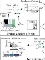
Western blotting is a universally used technique to identify specific proteins from a heterogeneous and complex mixture. However, there is no clear and common procedure to quantify the results obtained, resulting in variations due to the different software and protocols used in each laboratory. Here, we have developed a procedure based on the increase in chemiluminescent signal to obtain a representative value for each band to be quantified. Images were processed with ImageJ and subsequently compared using R software. The result is a linear regression model in which we use the slope of the signal increase within the combined linear range of detection to compare between samples. This approach allows to quantify and compare protein levels from different conditions in a simple and reproducible way.
Graphical overview

Background
Proteins are key biomolecules for the correct functioning of living animals; therefore, it is required not only to detect but also to accurately quantify them. Western blot is the most widely used and accepted method to detect proteins of interest using specific antibodies. Since the development of western blotting in 1979 (Towbin, H, PNAS 1979), more than 382,000 articles have been published using this technique (Western blot, PubMed, October 11, 2022). Since 2000, when 7,300 papers were published, there has been a constant increase in the number of articles reporting the use of this method (Moritz, 2020), reaching almost 22,600 in 2021. However, a proper quantification to determine the amount or the corresponding protein modification detected is still missing in most of the articles. In addition, reviewers and editors are eager to have trusty quantitative data regarding western blot analyses (Murphy and Lamb, 2013; Taylor et al., 2013;Janes, 2015; McDonough et al., 2015; Bass et al., 2017; Pillai-Kastoori et al., 2020). To assess accurate quantification, it is required to perform data normalization using proteins that do not vary due to experimental conditions. Usually, these are housekeeping proteins including actin, tubulin, and glyceraldehyde 3-phosphate dehydrogenase. Previous articles quantifying chemiluminescence western blots have relied on the use of single images of signals from different samples that are sometimes saturated, leading to incorrect outcomes. Fluorescence-based techniques using fluorophore-conjugated secondary antibodies are not commonly employed in most laboratories but provide a wider range of linear correlation between signal and protein abundance (Huang et al., 2019). Therefore, it is urgent to establish a simple, reliable method to quantify western blot signals to draw accurate conclusions in the studies.
Here, we describe an improved, simple protocol for western blot quantification taking advantage of chemiluminescent detection by ccd cameras and ImageJ and R software. Different images with different exposure times were utilized to generate the linear range for each protein to be quantified. The advantage of our procedure is that the signals are quantified across an interval of different exposures within the linear range for all the samples, where the differences between them are constant. Comparison of the slopes obtained provides a more accurate representation of the relative amounts of proteins in different samples than would be achieved by comparing individual images.
Materials and Reagents
The following list provides examples of the materials and equipment that we routinely use in our laboratory. Reagents and equipment with similar specifications will work as well.
All the materials and reagents listed were handled and stored following manufacturer’s instructions.
Polyvinylidene difluoride transfer membranes, 0.2 µm (PVDF membranes) (Thermo Fisher Scientific, catalog number: 88520)
Whatman 3MM CHR paper (Cytiva, catalog number: 3030-335)
β-glycerophosphate (AppliChem, catalog number: A2253, CAS number: 819-83-0)
β-mercaptoethanol (VWR BHD Chemicals, catalog number: 25351.182, CAS number: 60-24-2)
Acrylamide-bis solution (BioAcryl-P 30%, 37.5:1) (Alfa Aesar, catalog number: J61505)
Ammonium persulfate (APS) (Sigma-Aldrich, catalog number: A3678, CAS number: 7727-54-0)
Aprotinin (Sigma-Aldrich, catalog number: A1153, CAS Number: 9087-70-1)
BCA protein assay: reagent A (Thermo, catalog number: 23228) and reagent B (Thermo, catalog number: 23224)
Bis-Tris ultrapure (Thermo Fisher Scientific, catalog number: J12112.22, CAS number: 6976-37-0)
Bovine serum albumin (BSA) (Sigma-Aldrich, catalog number: A7906, CAS number: 9048-46-8)
Bromophenol blue (Amresco, catalog number: 0449-25G, CAS number: 115-39-9)
Dye reagent concentrate (Bio-Rad, catalog number: 500-0006)
Ethylenediaminetetraacetic acid (EDTA) (VWR Life Science, BHD Prolabo Chemicals, catalog number: 443885J, CAS number: 6381-92-6)
Glycerol (Thermo Fisher Scientific, catalog number: BP229-1, CAS number: 56-81-5)
Glycine (Sigma-Aldrich, catalog number: G8898-1KG, CAS number: 56-40-6)
HRP-conjugated anti-mouse antibody (Jackson ImmunoResearch, catalog number: 115-035-003, concentration used: 1:5,000)
HRP-conjugated anti-rabbit antibody (Jackson ImmunoResearch, catalog number: 111-035-003, concentration used: 1:5,000)
Hydrochloric acid (HCl) (Thermo Fisher Scientific, catalog number: H/1200/PB15, CAS number: 7647-01-0)
Isopropanol (Sigma-Aldrich, catalog number: 1.09634.1011, CAS number: 67-63-0)
Leupeptin (Sigma-Aldrich, catalog number: L9783, CAS number: 24125-16-4)
MES-SDS running buffer (Thermo Fisher Scientific, catalog number: NP0002)
Methanol (Fisher Chemical, catalog number: M/4000/PB17, CAS number: 67-56-1)
N,N,N',N'-tetramethyl-ethane-1,2-diamine (TEMED) (Thermo Fisher Scientific, catalog number: BP150-20, CAS number: 110-18-9)
Non-fat dry milk (Nestlé Sveltesse)
NP-40 (IGEPAL CA-630) (Sigma-Aldrich, catalog number: I3021, CAS number: 9002-93-1)
Phenylmethanesulfonyl fluoride (PMSF) (CalbioChem, catalog number: 52332, CAS number: 329-98-6)
Sodium azide (MERK, catalog number: 1066880100, CAS number: 26628-22-8)
Sodium chloride (NaCl) (Sigma-Aldrich, catalog number: 71383-5KG, CAS number: 7647-14-5)
Sodium dodecyl sulfate (SDS) (Bio-Rad, catalog number: 1610302, CAS number:151-21-3)
Sodium fluoride (NaF) (Sigma-Aldrich, catalog number: S7920-100G, CAS number: 7681-49-4)
Sodium orthovanadate (Sigma-Aldrich, catalog number: S6508, CAS number: 13721-39-6)
Trizma base (Tris) (Sigma-Aldrich, catalog number: T1503-1KG, CAS number: 77-86-1)
Tween-20 (Sigma-Aldrich, catalog number: P5927, CAS number: 9005-64-5)
WesternBrightTM ECL HRP Substrate (Advansta, catalog number: K-12045-D50)
Lysis buffer (see Recipes)
5× Laemmli buffer (see Recipes)
Polyacrylamide gels (see Recipes)
Transfer buffer (see Recipes)
TBST washing buffer (see Recipes)
Primary antibody blocking solution (see Recipes)
Secondary antibody blocking solution (see Recipes)
Equipment
Mini-PROTEAN® Tetra Vertical Electrophoresis Cell, 4-gel, for 1.0 mm thick handcast gels (Bio-Rad Laboratories Inc., catalog number: 1658001FC)
Mini-PROTEAN Tetra Companion Running Module (Bio-Rad Laboratories Inc., catalog number: 1658038)
Casting frame (Bio-Rad Laboratories Inc., catalog number: 1653304)
Casting stand gaskets (Bio-Rad Laboratories Inc., catalog number: 1653305)
Glass plates (Bio-Rad Laboratories Inc., catalog number: 1653311)
Short plates (Bio-Rad Laboratories Inc., catalog number: 1653308)
Combs, 15-well, 1.0 mm (Bio-Rad Laboratories Inc., catalog number: 1653360)
Buffer tank and lid with power cables (Bio-Rad Laboratories Inc., catalog number: 1658040)
Gel releasers (Bio-Rad Laboratories Inc., catalog number: 1653320)
Blot roller (Bio-Rad Laboratories Inc.)
Power supply (VWR, catalog number: HITAK622113)
MicroChemi System (Bio-Imaging Systems)
Software
ImageJ and R software
Procedure
The composition of solutions and buffers used are shown below under the section “Recipes”.
Western blot
Since this protocol aims to quantify the signal from membranes, we provide here a general western blotting guideline, based on which each user should apply the optimal conditions for his or her interest. In brief, proteins are electrophoretically separated in an acrylamide gel according to their size and then transferred to a membrane, to be probed with antibodies that recognize specifically antigenic epitopes displayed by the target protein.
The steps are the following:
Extract proteins from HEK293FT cells (at 80% confluency) seeded in a 6 cm plate adding 500 µL of cold lysis buffer with protease inhibitors and incubate for 30 min at 4 °C with gentle shaking. Collect the solution with the cells in a cold Eppendorf tube and centrifuge at 16,000× g for 10 min at 4 °C.
Note: To avoid protein degradation, include protease inhibitors and work in cold conditions, at 4 °C. Lysis can be performed using different lysis buffers including RIPA if e.g., immunoprecipitation will be performed.
Quantify protein concentration.
Note: Quantification of proteins needs to be done with an appropriate method depending on the lysis buffer used, i.e., BCA protein assay (for SDS-containing lysis buffer) and protein assay dye reagent concentrate (lysis buffer without SDS).
Collect the desired quantity of lysates (15–50 µg) in a new Eppendorf, add Laemmli buffer to a final 2× concentration up to 25 µL of volume, and mix well. Then, boil samples at 100 °C for 6 min, let them cool at room temperature and centrifuge at 16,000× g for 30 s.
Note: Samples can be stored at -20 °C if not used immediately.
Load the desired quantity of protein lysates in the corresponding acrylamide gel to perform SDS-PAGE. Place the gel in the tank filled with MES-SDS running buffer and apply current to allow protein separation until the front dye reaches the bottom of the gel (Figure 1).
Note: Depending on the size and proteins to be detected, the percentage and kind of acrylamide gels to be used will be different. For example, to detect proteins with high molecular weight (above 80 kDa), 6%–8% acrylamide gels are preferred. In case it is necessary to detect low (below 30 kDa) and high molecular weight proteins in the same gel, it is recommended to use gradient gels with a percentage of acrylamide from 4% to 12%. Depending on whether the acrylamide gel is a Bis-Tris or Tris-Glycine, the resolving range and the time required to run the samples will vary (30–40 min in Bis-Tris gels at 200 V to 75–120 min in Tris-Glycine gels at 90 V).
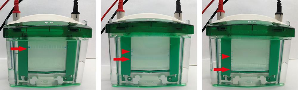
Figure 1. SDS-PAGE gel running; at loading (left panel) and after running for 30 min (middle panel) and 90 min (right panel). Note the molecular weight standards (blue) appearing on the left and right edges once the samples have run. Arrows point to the front dye and arrowheads to 75 kDa molecular weight marker.Transfer proteins from gel to PVDF membranes. Before obtaining the gel, label and activate the PVDF membrane by soaking it in methanol for a few seconds, rinse twice with ddH 2 O for 3–4 min, and incubate with transfer buffer until use. Stop current once the front dye has reached the bottom part of the gel. Assemble the transfer cassette in a container with transfer buffer as shown in Video 1.
Note: It is crucial to avoid air bubbles when setting the cassette by covering the sponge, Whatman paper, and the gel with transfer buffer. Failure to remove air bubbles in the assembled cassette will jeopardize the detection of proteins. After placing each component, remember to run the blot roller gently to avoid the presence of air bubbles during the transfer. Be careful with the orientation of the gel so as not to lose the order in which the samples were loaded; a different volume of molecular weight marker can be added in the first and last lane to aid this purpose.
 Video 1. Transfer preparation
Place the cassette in the frame in the right orientation located in the chamber filled with transfer buffer and an ice package. Include a magnetic stirrer and stir while applying a 200–400 mA current for at least 1.5 h in a cold room to avoid overheating. After that, remove PVDF membrane with the proteins attached and start the procedure to detect them.
Note: Protein transfer from gel to membrane can be done with different equipment, including semi-dry transfer. Insertion of the cassette in the wrong orientation will make proteins from the gel to migrate in the opposite direction of the PVDF membrane; therefore, proteins will be lost.
Block membrane with blocking solution with agitation for at least 30 min at room temperature.
Note: Blocking solution will depend on the primary antibody to be used. Check manufacturer datasheet for that info.
Incubate the membrane with the primary antibody in blocking solution with agitation for 2–3 h at room temperature or overnight at 4 °C.
Note: The quality of the signal and the amount of background will depend in a great manner on the quality/affinity of the antibodies. If possible, use antibodies that have been previously tested by you or other laboratories.
Wash with gentle agitation at least three times with TBST solution for at least 15 min, block membrane using TBST + 5% non-fat milk for 10 min with agitation, add the corresponding secondary antibody conjugated with HRP, and incubate for at least 45 min.
Note: The secondary antibody to be used can be coupled with different fluorophores instead of HRP, but extra care must be taken with light to avoid bleaching of signal.
Repeat the washes with TBST and leave the membrane in this solution until development.
Set up the settings for image acquisition in the MicroChemi apparatus using different exposure times.
Note: Acquisition of images can be performed with other equipment. The exposure times will depend on the quantity of protein and/or selectivity of the primary antibody. Routinely, we set time differences between exposures in the Chemidoc program of 1, 3, 5, 15, 30, 60, 180, 300, 600, and 900 s. The signal of each image corresponds to the accumulated time from the beginning, i.e., images 3 and 4 will have an exposure of 9 and 24 s, respectively.
Incubate membrane with the WesternBrightTM ECL HRP Substrate for 1 min.
Place the membrane in the MicroChemi chamber and acquire images (Figure 2).
Note: At the end of the experiment, take a picture with bright light to save an image with the molecular weight markers position in the membrane. This will help identifying the bands of interest.
Copy images and transfer to a computer with ImageJ program to process them.
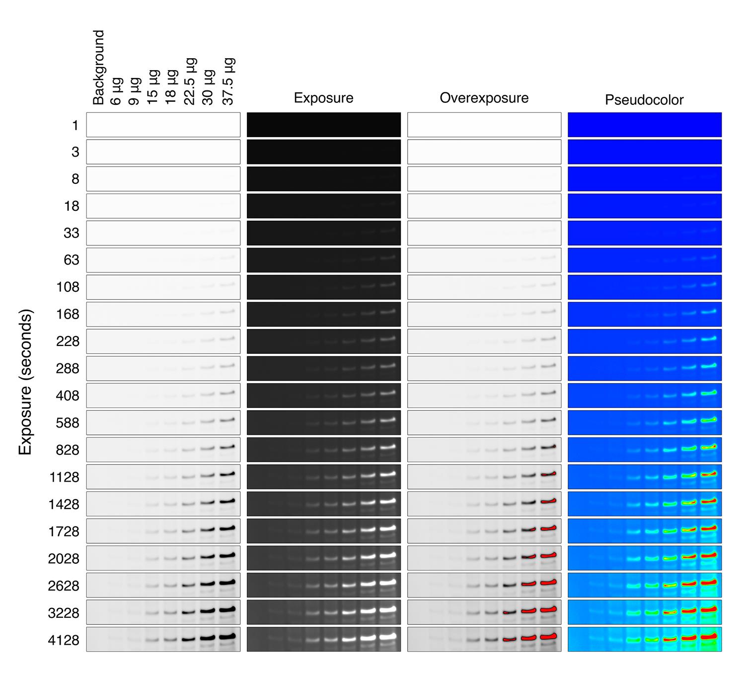
Figure 2. Images obtained with MicroChemi equipment and GelCapture software. Western blots for actin in HEK293FT cell lysates with different exposure times (from 1 to 4,128 s) showing original images (two left panels, the first being inverted), saturation image profile (third panel from the left), and pseudo color image (fourth panel from the left). Note that the signal becomes saturated (red signal) in 37.5 µg sample with 828 s of exposure.
Image processing and band quantification
The aim is to obtain a numerical value for the intensity of each band in each image captured during membrane exposure, using the analysis tools of ImageJ program (Video 2).
Video 2. Band quantificationOpen all images using ImageJ with the commands: File > Import > Image Sequence… choosing the folder directory where the images are located, the first one to start with, and the number of photos to import.
Note: Do not include the “Molecular Weight Markers Picture” taken with clear light, only the ones acquired with chemiluminescence.
Choose the parameters of interest to be recorded from the images. To do this, select Analyze > Set Measurements… clicking the ones that ImageJ should record for the analysis.
Note: In our case, we have selected Area, Mean gray value, Integrated density, and Display label. The analysis is going to be performed with Integrated density values, but as many parameters as desired can be recorded.
Select an image with visible bands, but not saturated (Figure 2, overexposure images), and delimit a rectangle that fits one of them with the "Rectangle" tool. Then, move the rectangle over an area of the membrane close to the bands but without signal, to capture the background. Record the measurements with the commands: Image > Stacks > Measure Stack…
Note: The less the area of the rectangle fits the band, the greater the possibility of introducing deviations due to the background (Gassmann et al., 2009). The size of the rectangle should not be modified, so that the same area is always quantified for all bands. If there are free wells in the gel, a lane with the same lysis buffer and Laemmli buffer can be included, which will serve to quantify the background.
Move the rectangle over each band and repeat the same commands to obtain measurements. As a result, a table with all the values collected for each of the bands in each sequence image will appear.
Note: Consider the order in which the bands have been quantified to know to which of the samples the value corresponds.
Save the data in .csv format with the commands File > Save As…
Linear model optimization
The aim of the analysis is to obtain a representative value for each band in the western blot. This value will be the slope of the signal increment within the linear range of the selected band.
Load the required packages for R software to work.
Note: If the packages are not installed, the command install.packages() needs to be used before loading them.
my_packages <- c("dplyr", "ggplot2", "openxlsx")
lapply(my_packages, require, character.only = TRUE)Set the working directory, the folders where the data file is located, and where the result of the analysis is going to be exported.
Note: Remember that quotation marks should be used.
WorkingDirectory <- "/Users/xxxxx/Desktop/Folder1/Folder2/Actin"
setwd(WorkingDirectory)Load the data from the image analysis in .csv format, copying the file name in the corresponding lane.
Note: Quotation marks should be used.
File_Name <- "Results.csv"
Results <- read.table(file = File_Name, sep = ",", header = T)Define the conditions of the experiment: the background and the samples that have been loaded on the gel. The script is going to assign each name to each set of measurements in a new column called “conditions”.
Note: Be careful to write them in the same order in which the quantification has been done from the images and use quotation marks so that R interprets them as text.
conditions <- c("Background", "6μg", "9μg", "15μg", "18μg", "22.5μg", "30μg", "37.5μg")
Results$Conditions <- factor(x = rep(conditions, each = max(Results$Slice)), levels = conditions)Introduce the exposure time for each image that has been quantified. The script is going to assign each value to its corresponding image in a new column called “Exposure.”
Note: Remember that it is not the value that has been introduced in the Chemidoc software, but the accumulated time from the beginning. The units to be used can be seconds or minutes; if using minutes, convert the values to decimal system and use “.” for decimals.
Exposure <- c(1, 3, 8, 18, 33, 63, 108, 168, 228, 288, 408, 588, 828, 1128, 1428, 1728, 2028, 2628, 3228, 4128)
Results$Exposure <- rep(exposure, times = length(conditions))Perform background correction. The code will subtract the signal from the background of each image in all analyzed bands. The result will be written in a new column called “BckgCorrect.”
Results$BckgCorrect <- rep(0, dim(Results)[1])
for (i in 1 :dim(Results)[1]) {
Bkgnd <- Results$Conditions == "Background" & Results$Exposure == Results[i,"Exposure"]
Results$BckgCorrect[i] <- Results[i,"IntDen"] - Results[Bkgnd,"IntDen"]
}Represent the data in a scatterplot, with the exposure time as the independent variable and the background corrected signal as the dependent one (Figure 3). The purpose of the graph is to determine visually the linear range for the increment of the signal.
ggplot(Results, aes(x = Exposure, y = BckgCorrect, color = Conditions))+
geom_point() + geom_line() + theme_classic()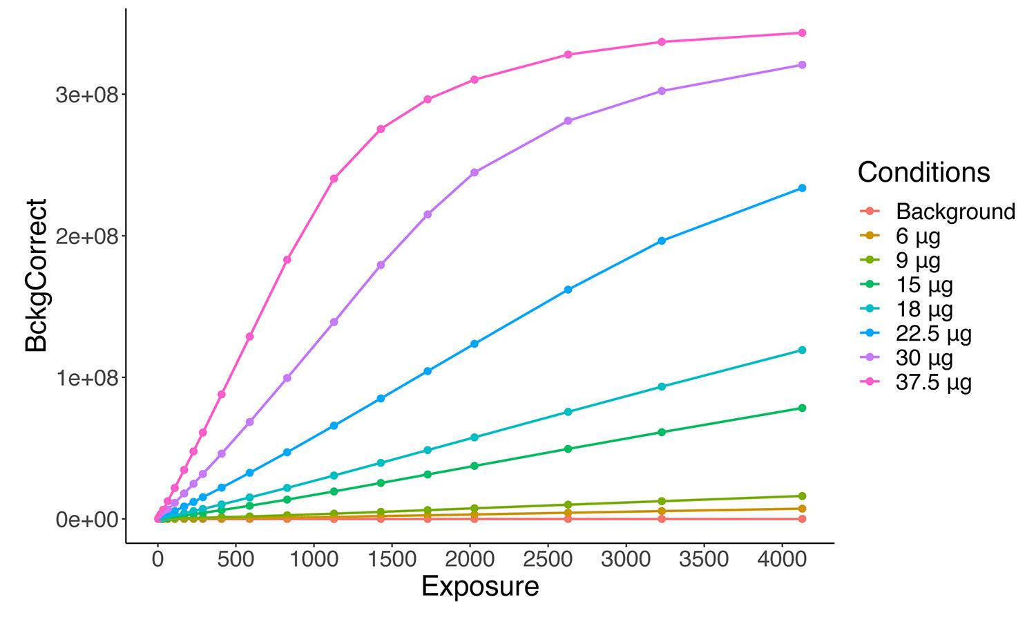
Figure 3. Representation of band quantifications. The signal of each band (y-axis) with respect to the exposure time (x-axis) is shown. Note that in the samples with higher protein content (22.5, 30, and 37.5 µg) the linearity between exposure time and signal is lost at certain exposure time.Optimize the model by manually selecting the first and last exposure time to be considered that stays within the linear range for all conditions of interest. The script will define a new data frame with the filtered data between these two points, named “Results_filtered.”
First_Expossure = 63
Last_Expossure= 828
Results %>% filter(between(Exposure, First_Expossure, Last_Expossure)) -> Results_filteredBuild the linear model using simple linear regression, with exposure time as predictor variable and corrected signal as response variable. The script will calculate the regression parameters for each condition of the experiment, obtaining a new data frame with the value of the slope of the regression line, the R-squared coefficient of determination to evaluate the goodness of fit, and the p-value to evaluate its statistical significance (Table 1). It will also generate a new scatterplot with the filtered data (Figure 4).
<- data.frame(t(mapply(unlist, by(Results_filtered, Results_filtered$Conditions, function (x) summary(lm(BckgCorrect~Exposure, x)))))) %>%
select(slope = coefficients2, adj.r.squared, p.value = coefficients8)
ggplot(Results_filtered, aes(x = Exposure, y = BckgCorrect, color = Conditions))+
geom_point() + geom_line() + theme_classic()
knitr::kable(Results_model)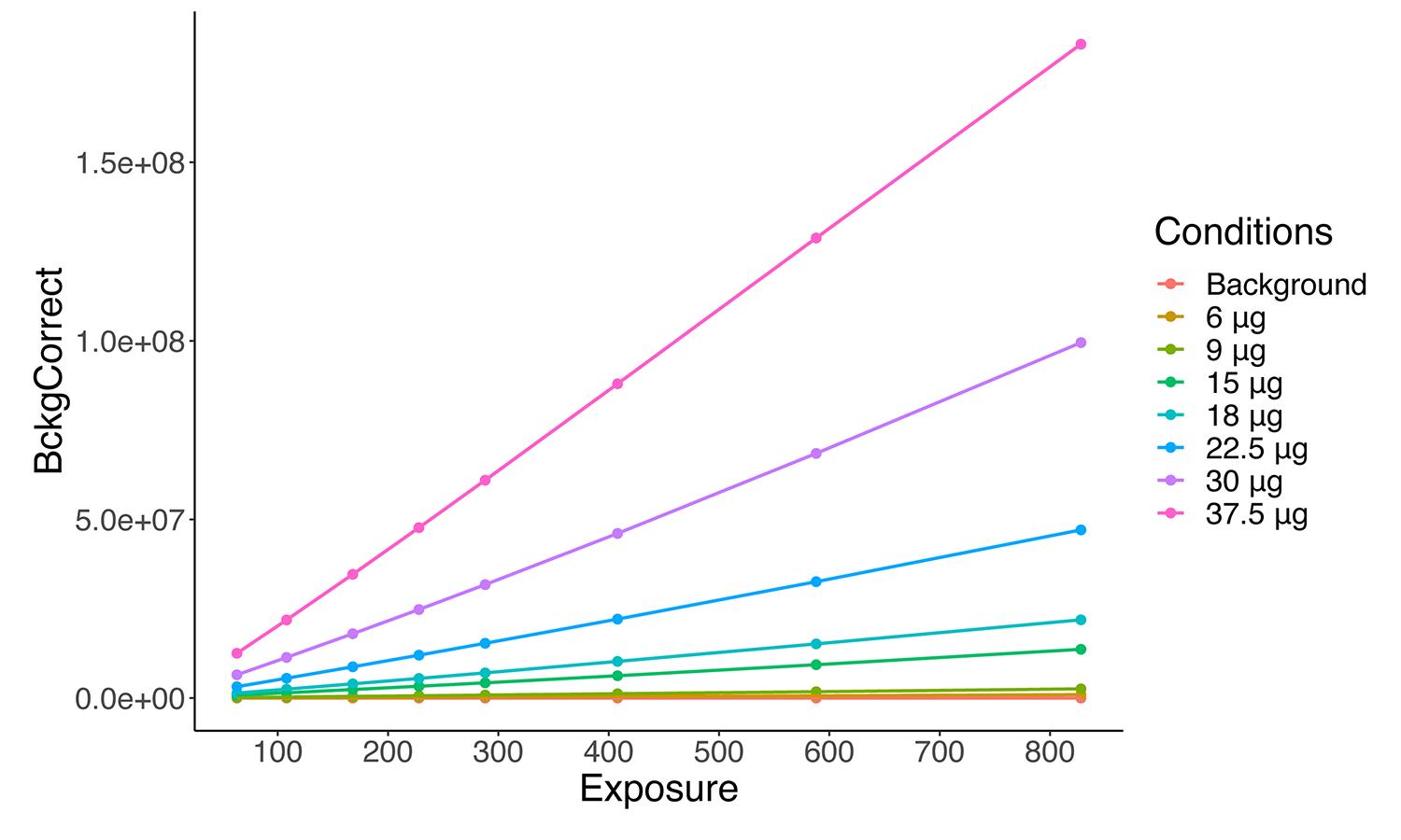
Figure 4. Adjusted representation of band quantifications. After removing the samples with lower and/or higher exposure (in which linearity was lost), linearity for different amounts is kept and will allow to accurately calculate the slope for each concentration.Table 1. Regression parameters for each condition of the experiment
Conditions Slope Adj. r. squared p. value Background 0 NaN NaN 6 μg 1157.633 0.9988883 2.704757e-10 9 μg 3156.074 0.9993988 4.277239e-11 15 μg 16760.63 0.9986983 4.34215e-10 18 μg 26829.65 0.9994091 4.061036e-11 22.5 μg 57338.1 0.9993725 4.864208e-11 30 μg 121563.9 0.9989834 2.068317e-10 37.5 μg 223579.3 0.9998507 6.546559e-13 If the regression coefficient is not close enough to 1 and/or the scatterplot does not fit the linear range, go back to step C8, and adjust the exposure values again.
Export the analysis results. The script will overwrite the initial excel file, saving all the data in a sheet named “DATA,” the filtered data between exposure times in a sheet named “DATA_FILTERED,” and the coefficients of the linear model in a sheet named “MODEL.”
Note: Remember that these are chemiluminescent signal values. Western blotting is a semiquantitative technique, so the next step in interpreting the results should be to compare these values with a housekeeping or a reference protein (protein of interest/reference protein).
write.xlsx(list(DATA = Results, DATA_FILTERED = Results_filtered, MODEL = Results_model), file = "File_Name", row.names = T)
Example
As an example of the method described here, complementary to that published in Sánchez-Sánchez et al. (2023), we show the quantification of TrkA activation after stimulation with nerve growth factor (NGF) for different times. Briefly, we used primary cultures of sensory neurons enriched in TrkA-positive neurons selected with NGF for 5–6 days. We then deprived the culture of neurotrophin for 4 h and stimulated with NGF (50 ng/mL) for the corresponding time. We collected cell lysates and performed western blotting using pTrkA (for activated receptor) (Figure 5A, left panels) and TrkA (Figure 5B, left panels) antibodies, taking the top 140 kDa band as the reference protein. We quantified the signals from the pTrkA and TrkA bands as described in this protocol. We measured the signal intensity of different images for each sample (Figures 5A and 5B, exposure blots) and, together with the exposure time settings, defined the combined linear range for each protein (Figures 5A and 5B, right plots). As described above, we built a linear regression model. We used the slope as a representative value to calculate the ratio of pTrk to TrkA and plotted the results of independent experiments (Figure 5C).
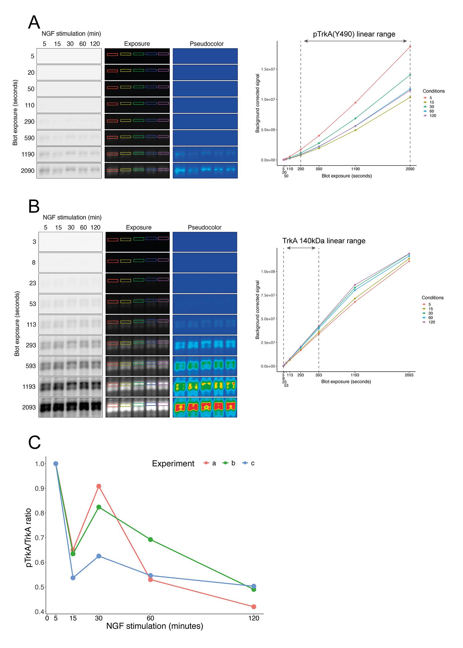
Figure 5. Example of signal quantification. Images with different exposures showing pTrkA (panel A) and TrkA (panel B) signals were quantified in cultured sensory neurons after NGF stimulation for different stimulation times. The colored rectangles in both panels represent the membrane areas used for quantification. A rectangle of another region without signal was utilized as background (not shown in the images). Note that saturation can be detected at higher exposures of the TrkA blot in the pseudo color images (red color). On the right side of each panel there is a graph showing the signal increase curve for each time point. The range between dashed lines indicates the exposures taken to optimize the linear regression model and to perform the quantification within linearity. Note that the saturation in the pseudo color images matches the flattering of the curves in the plots. (C) Quantification of TrkA activation (pTrkA/TrkA ratio). Normalization was performed using the 5 min time point of NGF stimulation. Each colored line represents the results obtained in a single experiment (n = 3). Panels A and B correspond to experiment c in panel C.Useful tips
It is important to include control and experimental/problem samples in the same membrane, to be able to compare since there is always some variability between membranes, even with those carried out in parallel for the whole experiment.
Total protein to be loaded in the gel (usually between 15 and 50 µg) will depend on the abundance of the protein of interest to be detected and the affinity of the antibodies to be used. Loading an excess of total protein can also saturate the membrane during the transfer, and differences between samples could be misleading.
Remember that western blot is a semiquantitative technique and a loading control, housekeeping protein, or reference protein are always needed to normalize the data.
The quality of the signal and the amount of background will depend in a great manner on the quality/affinity of the antibodies. If possible, use antibodies that have been previously tested by you or other laboratories.
When working with R software, do not forget to use quotation marks in what should be text.
Recipes
The following solutions/buffers are obtained using the quantities indicated, and the final concentration of each component is given in brackets.
Lysis buffer
2.42 g of Trizma base pH 8.0 (20 mM)
8 g of NaCl (137 mM)
10 mL of NP-40 (1%)
Ultrapure MilliQ water up to 1 L
Store at 4 °C
Just prior to use, add the corresponding volume to have a final concentration of 1 mM PMSF, 1 μg/mL aprotinin, 2 μg/mL leupeptin, 1 mM sodium orthovanadate, 10 mM NaF, and 20 mM β-glycerophosphate.
5× Laemmli buffer
30.29 g of Trizma base pH 6.8 (250 mM)
100 g of SDS (10%)
500 mL of glycerol (50%)
67 mg of bromophenol blue (0.01%)
39.07 g of β-mercaptoethanol (500 mM)
Ultrapure MilliQ water up to 1 L
Stored at -20 °C
Polyacrylamide gels
Acrylamide-bis solution up to the desired percentage, 350 mM Bis-Tris buffer pH 6.4, 0.1% SDS, ultrapure MilliQ water, APS (0.1%), and TEMED (6.6 mM). Mix the reagents in that order and avoid bubbles to prevent patchy polymerization. Prepare 4.5 mL of final volume per resolution gel, and 2 mL with lower acrylamide percentage for the stacking. The use of a thin layer of isopropanol to avoid contact with oxygen during polymerization of the resolving gel also helps to avoid bubbles and to have a clean separation with stacking. Homemade gels can be stored up to 3–4 days at 4 °C in a humid chamber.
Transfer buffer
5.8 g of Trizma base pH 8.3 (25 mM)
2.9 g of glycine (192 mM)
100 mL of methanol (10%)
Ultrapure MilliQ water up to 1 L and adjust pH
Store at 4 °C and reuse up to five times
TBST washing buffer
1.21 g of Trizma base pH 7.5 (10 mM)
8.8 g of NaCl (150 mM)
0.32 g of EDTA (1 mM)
10 mL of Tween-20 (0.1%)
Ultrapure MilliQ water up to 1 L and adjust pH
Primary antibody blocking solution
100 mL of TBST washing buffer
3 g of BSA (3%)
32.5 mg of sodium azide (0.05%)
Stored at 4 °C
Secondary antibody blocking solution
100 mL of TBST washing buffer
5 g of non-fat dry milk (5%)
Prepare just before use with gentle agitation to avoid foaming
Acknowledgments
We thank Deogracias’ and Arevalo’s lab for input into the manuscript. This work was supported by grant PID2020-113130RB-100 funded by MCIN/AEI/10.13039/501100011033 and by the European Union to J.C.A. D.C.G was granted by Consejería de Educación Junta de Castilla y León and the European Social Fund.
Competing interests
The authors declare no competing interests and mentioning of specific materials, reagents, and equipment does not imply endorsement by the funding agencies.
References
Bass, J. J., Wilkinson, D. J., Rankin, D., Phillips, B. E., Szewczyk, N. J., Smith, K. and Atherton, P. J. (2017). An overview of technical considerations for Western blotting applications to physiological research. Scand J Med Sci Sports 27(1): 4-25.
- Gassmann, M., Grenacher, B., Rohde, B. and Vogel, J. (2009). Quantifying Western blots: pitfalls of densitometry. Electrophoresis 30(11): 1845-1855.
- Huang, Y. T., van der Hoorn, D., Ledahawsky, L. M., Motyl, A. A. L., Jordan, C. Y., Gillingwater, T. H. and Groen, E. J. N. (2019). Robust Comparison of Protein Levels Across Tissues and Throughout Development Using Standardized Quantitative Western Blotting. J Vis Exp(146). doi: 10.3791/59438.
- Janes, K. A. (2015). An analysis of critical factors for quantitative immunoblotting. Sci Signal 8(371): rs2.
- McDonough, A. A., Veiras, L. C., Minas, J. N. and Ralph, D. L. (2015). Considerations when quantitating protein abundance by immunoblot. Am J Physiol Cell Physiolv 308(6): C426-33.
- Moritz, C. P. (2020). 40 years Western blotting: A scientific birthday toast. J Proteomics 212: 103575.
- Murphy, R. M. and Lamb, G. D. (2013). Important considerations for protein analyses using antibody based techniques: down-sizing Western blotting up-sizes outcomes. J Physiol 591(23): 5823-31.
- Pillai-Kastoori, L., Schutz-Geschwender, A. R. and Harford, J. A. (2020). A systematic approach to quantitative Western blot analysis. Anal Biochem 593: 113608.
- Sánchez-Sánchez, J., Vicente-García, C., Cañada-García, D., Martín-Zanca, D. and Arévalo, J. C. (2023). ARMS/Kidins220 regulates nociception by controlling brain-derived neurotrophic factor secretion. Pain 164(3): 563-576.
- Taylor, S. C., Berkelman, T., Yadav, G. and Hammond, M. (2013). A defined methodology for reliable quantification of Western blot data. Mol Biotechnol 55(3): 217-226.
- Towbin, H., Staehelin, T. and Gordon, J. (1979). Electrophoretic transfer of proteins from polyacrylamide gels to nitrocellulose sheets: procedure and some applications. PNAS 76: 4350-4354.
Article Information
Publication history
Published: May 5, 2023
Copyright
© 2023 The Author(s); This is an open access article under the CC BY-NC license (https://creativecommons.org/licenses/by-nc/4.0/).
How to cite
CAÑADA GARCÍA, D. and Arévalo, J. C. (2023). A Simple, Reproducible Procedure for Chemiluminescent Western Blot Quantification. Bio-protocol 13(9): e4667. DOI: 10.21769/BioProtoc.4667.
Category
Biochemistry > Protein > Quantification
Molecular Biology > Protein > Detection
Do you have any questions about this protocol?
Post your question to gather feedback from the community. We will also invite the authors of this article to respond.
![]() Tips for asking effective questions
Tips for asking effective questions
+ Description
Write a detailed description. Include all information that will help others answer your question including experimental processes, conditions, and relevant images.