
- Submit a Protocol
- Receive Our Alerts
- EN

- Protocols

- Articles and Issues
- For Authors
- About
- Become a Reviewer

Expression Stability Analysis of Candidate References for Normalization of RT-qPCR Data Using RefSeeker R package
(*contributed equally to this work) Published: Vol 13, Iss 17, Sep 5, 2023 DOI: 10.21769/BioProtoc.4801 Views: 280
Reviewed by: AYŞE NUR PEKTAŞUte Angelika HoffmannHélène Léger
Original research article
The authors used this protocol in:

May 2023

Protocol Collections
Comprehensive collections of detailed, peer-reviewed protocols focusing on specific topics


Abstract
When performing expression analysis either for coding RNA (e.g., mRNA) or non-coding RNA (e.g., miRNA), reverse transcription quantitative real-time polymerase chain reaction (RT-qPCR) is a widely used method. To normalize these data, one or more stable endogenous references must be identified. RefFinder is an online web-based tool using four almost universally used algorithms for assessing candidate endogenous references—delta-Ct, BestKeeper, geNorm, and Normfinder. However, the online interface is presently cumbersome and time consuming. We developed an R package, RefSeeker, which performs easy and straightforward RefFinder analysis by enabling raw data import and calculation of stability from each of the algorithms and provides data output tools to create graphs and tables. This protocol uses RefSeeker R package for fast and simple RefFinder stability analysis.
Key features
• Perform stability analysis using five algorithms: Normfinder, geNorm, delta-Ct, BestKeeper, and RefFinder.
• Identification of endogenous references for normalization of RT-qPCR data.
• Create publication-ready graphs and tables output.
• Step-by-step guide dialog window for novice R users.
Graphical overview
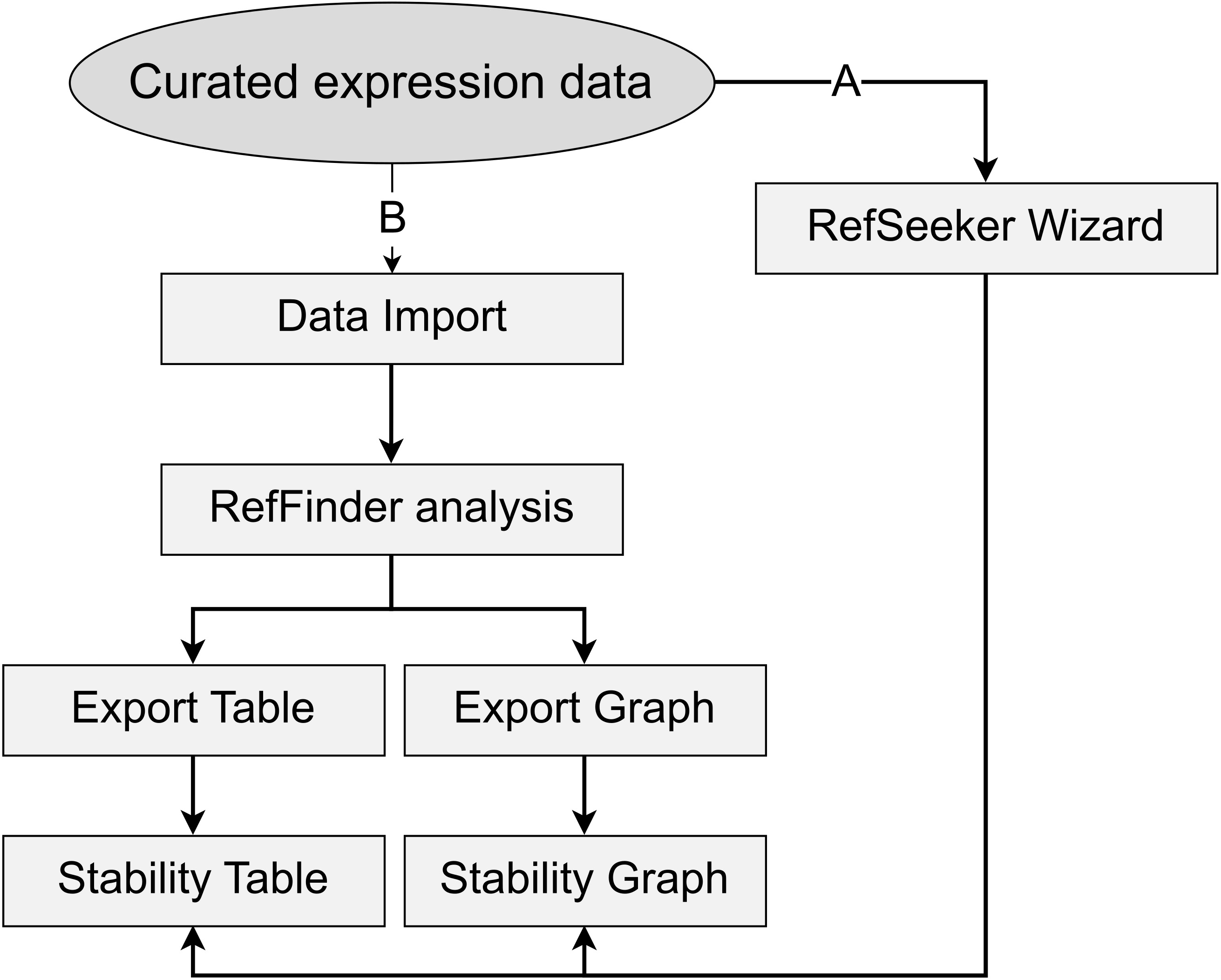
Simple workflow diagram. Two main workflow paths are presented. A) Using the RefSeeker wizard allows non-R programmers to easily load data and choose between selected output formats. B) Command line interface provides more options to control input and output formats and to automate analysis.
Background
Whether coding or non-coding, gene expression research represents a large field of investigation, including molecular biomarker research, drug research, cancer diagnostics, pathway research, RNA interference studies, stem cell research, and much more. In many of these fields, reverse transcription quantitative real-time polymerase chain reaction (RT-qPCR) is used to validate results and investigate changes in expression of a variety of RNA types. The Minimum Information for Publication of Quantitative Real-Time PCR Experiments (MIQE) guideline requirements have been widely adopted by the scientific community (Bustin et al., 2009). These guidelines assert that the use of three or more stably expressed endogenous references should be used for normalization of target RNAs (e.g., genes/mRNA or miRNAs). Additionally, these references should preferably be of the same type of RNA as the targets.
When performing expression analysis, it is often required to analyze the stabilities of reference genes used to normalize the data from targets of interest (Bustin et al., 2009). The selection of a sufficient number of adequately stable references, typically three or four, is a crucial step since the choice may significantly influence the results and could lead to wrong conclusions (Faraldi et al., 2019). Expression data is often obtained as a set of quantification cycle (Cq), crossing point (Cp), cycle threshold (Ct), or take-off point (TOP) values (Bustin et al., 2009). These expression values are typically obtained by performing the RNA quantification in technical triplicates or quadruplicates, averaging these data results in one value per RNA target (e.g., gene or miRNA) for each sample.
Four different algorithms are commonly used for identifying stable RNAs: (1) Normfinder calculates intra- and inter-group variations (Andersen et al., 2004); (2) geNorm uses an average pairwise standard deviation with all other candidates as the stability measure M (Vandesompele et al., 2002); (3) BestKeeper calculates a range of statistics but bases the individual stability on the mean absolute deviation of the raw Cp values (Pfaffl et al., 2004); and (4) the delta-Ct (ΔCt) method compares each candidate average standard deviation of ΔCt values for each combination of candidates (Silver et al., 2006). Further details on the different algorithms are beyond the scope of this protocol, and further information on their strengths and weaknesses can be found elsewhere (De Spiegelaere et al., 2015; Sundaram et al., 2019).
To deal with differences in results from these algorithms, Xie et. al. created RefFinder, which combines the rankings of the four algorithms and gives a geometric mean of these ranks (Xie et al., 2012 and 2022). RefFinder is available as an online tool, allowing researchers and others to perform the analysis by copying their expression data into a textbox and pressing the analyze button; results are then presented on the webpage.
Given that RefFinder is an online tool, data needs to be copied and pasted into a web-based interface. After the analysis, the results need to be copied and pasted back into a statistical or spreadsheet software of choice for further processing, table generation, and/or graphical depiction. This involves extensive manual work, especially in cases when multiple datasets are used simultaneously or when analyses need to be redone. Moreover, the process can be error prone, considering that copying and pasting manually to and from many different sources and destinations can be disorienting. Therefore, we aimed to develop a straightforward method to perform RefFinder analysis on preprocessed RT-qPCR data, providing easy generation of tables, datasheets, and graphical output: the RefSeeker package.
Software description
RefSeeker is a package developed in R designed to be compatible across different operating systems. R is a widely used, free, and open-source statistical environment, thus providing a great basis for expression data analysis (R Core Team, 2022). R provides great tools for working with data in tabular format as well as for plotting and graphing. The RefSeeker package utilizes widely available tools either available through base R or through The Comprehensive R Archive Network (CRAN).
As for RefFinder, to use the RefSeeker package, expression data need to be prepared in a tabular format. However, data can be prepared either as a data object prepared in R or as one of the supported file types (.xls, .xlsx, .ods, .csv, .tsv, or .txt). Each column represents a named target (gene, miRNA, or other) and each row represents a sample. If the data file is created using R, an index column might be added to the .csv file by default. This should be avoided by setting row.names = FALSE. In case of spreadsheets (Excel or .ods) where more than one dataset is included, each sheet in the spreadsheet file can contain a dataset. Naming the sheets will make it easier to identify the data later, since the name is carried over. In case of txt-based files, e.g., .csv, .tsv, or plain .txt tables, each dataset must be in a separate file in the same folder.
The package functions can be divided into four categories:
1. Data import functions, which import data from different sources (.csv, .tsv, .txt, .xls, .xlsx, and .ods) and arrange it for further processing. A wrapper function, rs_loaddata(), identifies the file extensions and calls the proper import function.
2. Data processing functions. RefSeeker uses four main functions to perform the RefFinder analysis: rs_normfinder(), rs_genorm(), rs_bestkeeper(), and rs_deltact(). These functions are all called by the rs_reffinder() function to determine stability rankings. The comprehensive rank is then calculated as the geometric mean of these stability rankings.
3. Data export functions for further analysis, visualization, and publication of results. The function rs_graph() handles printing and optionally exporting of graphs as .png, .tiff, .jpeg, or .svg file formats. Likewise, the function rs_exporttable() handles export of data tables, either as spreadsheets (.ods or .xlsx), txt-based formats (.csv, .tsv, .txt), or formatted tables in docx format.
4. Interactive implementation of the above functionality through the rs_wizard(). This function provides a graphical user interface dialog window for selecting data and output table and graphical formats.
See Figure 1 for an overview of the main functions and their association to the workflow.
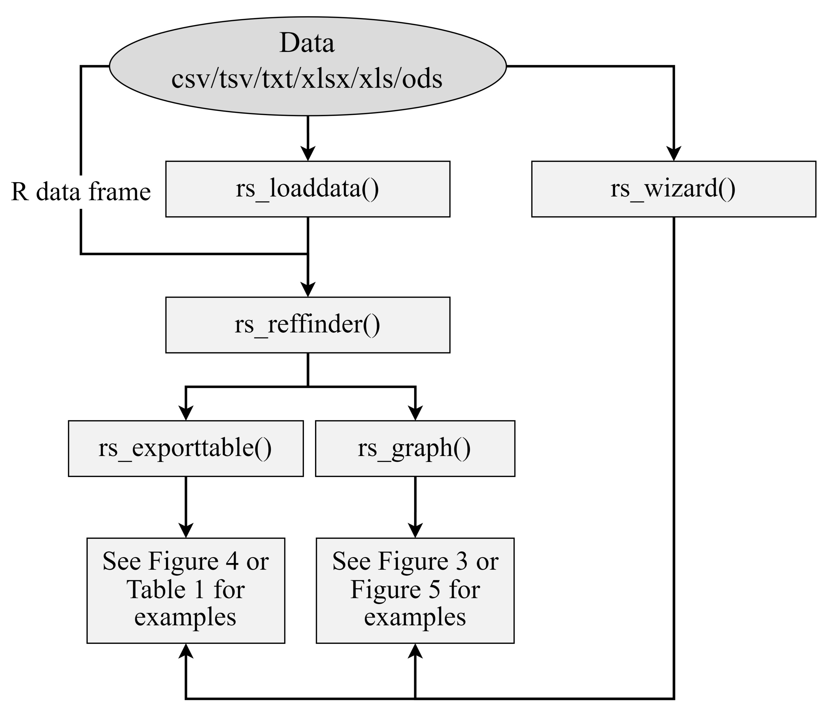
Figure 1. Simple data analysis workflow diagram. Data can be loaded from outside sources via the rs_load() or rs_wizard() functions. RefFinder analysis can be performed on the data using rs_reffinder(), and the analyzed data can be visualized and exported via the rs_exporttable() and rs_graph() functions. Examples of output can be seen in Figure 3, Figure 4, Figure 5, and Table 1.
Equipment
Computer with Windows, MacOS, or Linux-based operating system compatible with R (≥ 4.1.0)
Software and datasets
R software environment (≥ 4.1.0) (https://www.r-project.org/)
RStudio integrated development environment (≥ 1.4.0) (optional, https://rstudio.com/)
Datasets can be prepared in several ways, and processing of raw expression data is outside the scope of this protocol. However, in general, data should be cleaned, quality checked, and adjusted for interplate variability (Petersen et al., 2022).
Data can be prepared in either one of the supported file types (.xlsx, .ods, .csv, .tsv, or .txt) or as a data frame in R.
Sample data can be downloaded from: https://github.com/Hannibal83dk/RefSeeker/blob/main/SampleData/RefSeekerSampleData.xlsx (see Figure 2). These data have been previously described, and details about experiment design, data acquisition, and processing can be found in Petersen et al. (2022), from where the data have been obtained.
• No matter the input source, the following requirements are the same:
• Each column must be representing a gene/target and each row an individual sample*.
• Each column must be named.
• Row names must be excluded.
• No missing data is allowed**.
*Although the RefSeeker package can handle spaces and dashes in column names, some downstream R processes might not be able to. Best practices therefore recommend avoiding these characters in column names.
**Missing data can be handled in several ways. If samples need to be preserved, targets can be removed; if it is more desirable to keep targets, samples can be removed. If both are important, a percentage threshold for allowed missing data can be chosen. This threshold is individually selected; however, it should be as low as possible. A specific recommendation cannot be provided here; however, a threshold of 20% missing data has been used before and seems to be an approximate upper limit. Following target exclusion, remaining missing datapoints can be imputed using different tools [e.g., MissForest (missForrest package), k-Nearest Neighbor (VIM package), Multiple Imputation by Chained Equations (mice package), or max + 1 (manually implemented)].
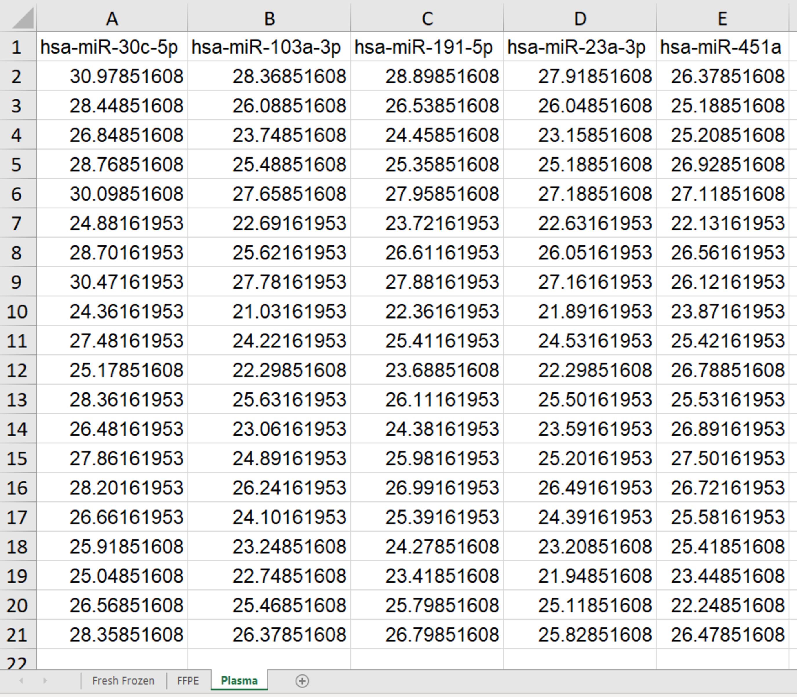
Figure 2. Example of expression data in an Excel file used for RefSeeker analysis. These may be averages of triplicates or quadruplicates and should be adjusted for e.g., possible interplate variation. Targets are given in the first row. Each of the following rows represents raw Cp values (adjusted for interplate variance) obtained from each sample. The file contains three spreadsheets: fresh frozen, formalin fixed and paraffin embedded (FFPE), and Plasma, each containing different datasets.
Procedure
Installing R and RStudio
The installation of R and RStudio are out of the scope of this protocol; however, more information on how to install these can be found on their respective websites:
R base: https://cran.r-project.org/
Installing dependencies
The RefSeeker has a few dependencies that need to be installed first by typing:
install.packages(c('ctrlGene', 'ggplot2', 'reshape2', 'readxl', 'openxlsx', 'data.table', 'readODS', 'flextable', 'officer'))
Installation of RefSeeker package
After installation of dependencies, the package can be installed in two ways:
Download Package Archive from GitHub:
Download the latest version of RefSeeker_latest.tar.gz file to your computer:
The latest version can be found at:
https://github.com/Hannibal83dk/RefSeeker/releases/latest/download/RefSeeker_latest.tar.gz
Open R or RStudio.
In the R Console, type:
install.packages("<PATH/TO/RefSeeker_latest.tar.gz>", repos = NULL, type = "source")
Note: Please note that the entire part of <PATH/TO/RefSeeker_latest.tar.gz> needs to be changed to the specific location of the downloaded file on your computer.
Alternatively, if RStudio is being used: from the menu bar, open the dropdown menu Tools > Install Packages > Select Package from Archive File in the Install from drop-down menu. Browse for the downloaded Package archive > press Install.
Use devtools to download from GitHub:
Make sure the devtools package is installed in your R environment. In the R Console, devtools can be installed from CRAN using:
install.packages("devtools")
In the R console type:
devtools::install_github("Hannibal83dk/RefSeeker", build_vignettes = TRUE)
RefFinder analysis
To illustrate the usability and ease of use of the package, three expression datasets with Cp data of six miRNAs from 20 patients in three sample types [Fresh frozen, formalin fixed and paraffin embedded (FFPE), and blood plasma] will be used (Petersen et al., 2022). The data are stored as individual sheets in an .xlsx file (Figure 2).
The aim is to identify the most stable miRNAs for normalization for each dataset. Firstly, the package needs to be loaded into an R environment. Two options are available for analysis.
Quick all-in-one analysis wizard:
Load the RefSeeker package:
In the R console first type:
library(RefSeeker)
Running the RefSeeker wizard will open a graphical interface dialog window, providing quick selection of input data and output formats.
Now, run the following in the console:
rs_wizard()
This will result in a dialog window popping up (see Figure 3).
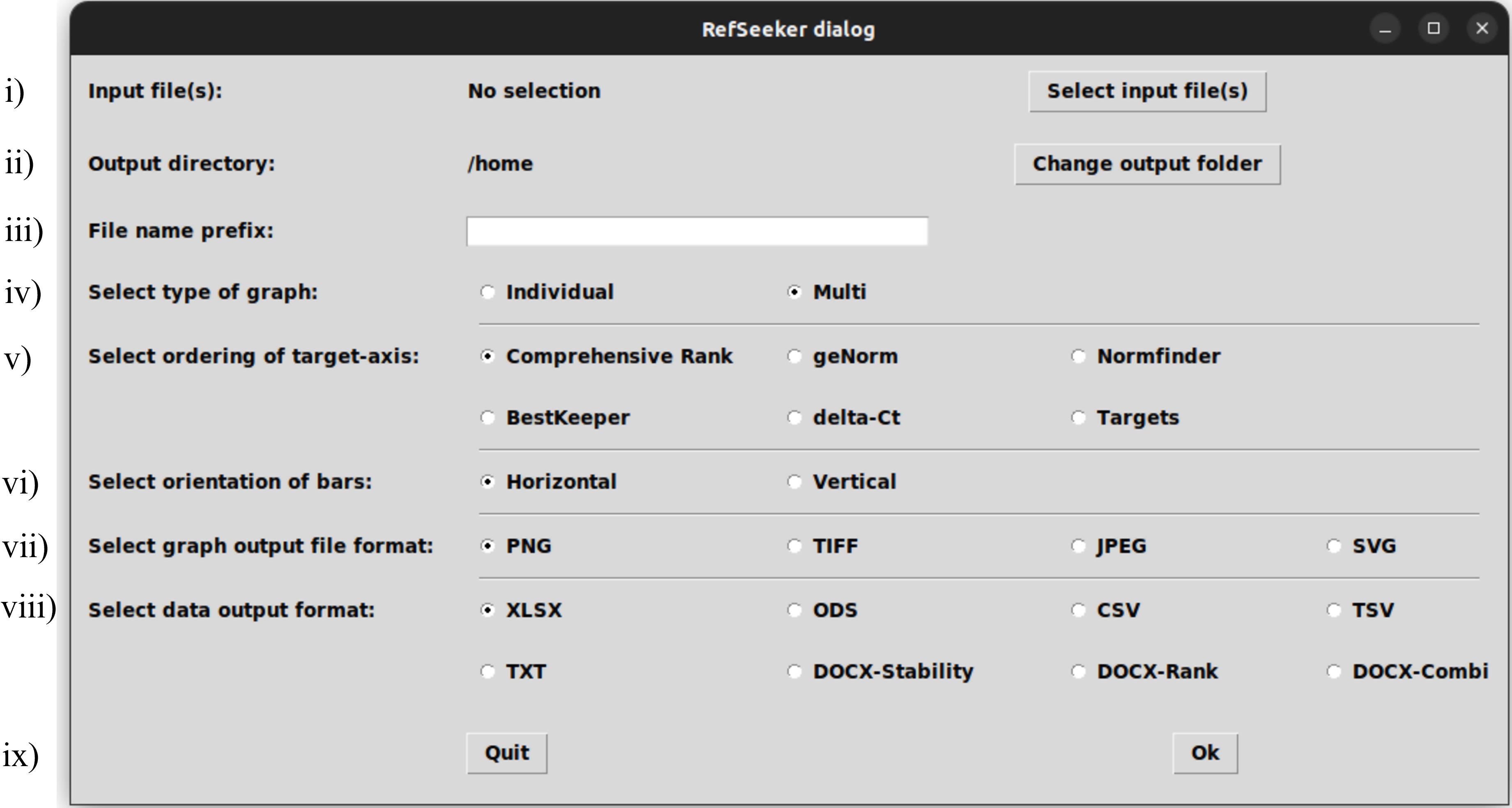
Figure 3. The rs_wizard() dialog allowing interactive quick analysis. The dialog consists of nine sections: i) selection of input file(s), ii) selection of folder for output files, iii) optional prefix for output file names, iv) selection of bar graph format, v) selection of order of the target axis, vi) selection of the orientation of the bar graph, vii) selection of the graph output file format, viii) selection of the table format, and ix) option for proceeding or quitting the analysis.Pressing the Select input files button (Figure 3-i) will open a file manager. From here, navigate to the .xlsx file and select it.
Press the Change output folder button (Figure 3-ii) and select an output directory from the file manager.
A file name prefix can be selected to identify the output files (Figure 3-iii). From the radio buttons, the desired output can be modified.
First, select the desired type of graph (Figure 3-iv): Individual will make a graph for each dataset and Multi will create a faceted graph combining all datasets in one graph (see Figure 4).
The ordering of the x-axis can also be changed (Figure 3-v). This defaults to Comprehensive Rank, meaning that all the target arrangements on the x-axis will be ordered from most to least stable, based on the ranking provided by the comprehensive rank.
The desired direction of the bar plot can be selected (Figure 3-vi).
Select desired file format to output the graph (Figure 3-vii).
Lastly, select the desired table output format (Figure 3-viii).
Press Ok and collect your outputs in the selected output folder (Figure 3-ix).
From the default selections, a .png file and an .xlsx file will be created in the output folder selected (Figure 4 and Figure 5). In step D1i (Figure 3-viii), a docx type table can be selected instead of the .xlsx file. An example of a docx type table format can be seen in Table 1. This is a good choice for presenting stabilities in a publication.
From the generated output (Figure 4 and Figure 5), targets with lower stability values are considered more stable. It is seen that the most stable endogenous miRNAs are hsa-miR-191-5p and hsa-miR-23a-3p for plasma, hsa-miR-23a-3p and hsa-miR-30c-3p for fresh frozen tissue, and hsa-miR-30c-3p ahashsa-miR-191-5p for FFPE tissue. Note that, since the different algorithms evaluate stability differently, results may vary between these (De Spiegelaere et al., 2015). Since BestKeeper only evaluates standard deviations of each sample, it is common to observe high differences between BestKeeper and the other algorithms that are more interdependent, especially GeNorm and delta-Ct, which evaluate highly correlated targets as more stable. Sundaram et al. (2019) suggests an integrated approach to this problem by removing targets with high overall variance before performing the analysis again.
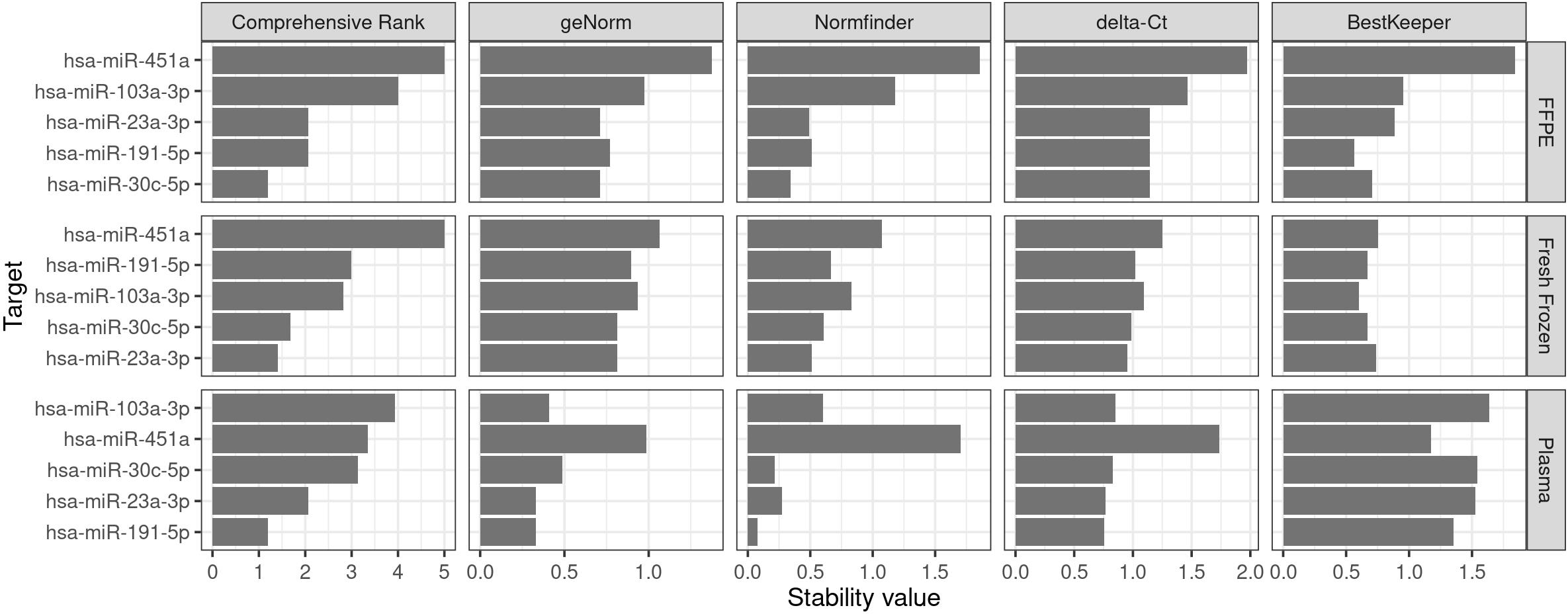
Figure 4. Example of graph output created using RefSeeker. A multi graph with data from three different datasets using horizontal layout and targets sorted by the Comprehensive Rank.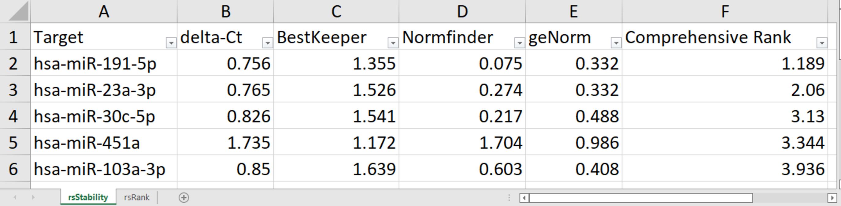
Figure 5. Example of Excel table output. Stability values from each algorithm are provided in the first sheet and targets are ordered by the Comprehensive Rank. The second sheet is similar to the first but contains rankings instead of stability values.Table 1. Example of docx-Combi type table output format
Plasma
delta-Ct
BestKeeper
Normfinder
geNorm
Comprehensive Rank
Target
Avg. STDEV.
Rank
MAD
Rank
Stability
Rank
Avg.M
Rank
Geom. mean value
Rank
hsa-miR-191-5p
0.756
1
1.355
2
0.075
1
0.332
1
1.189
1
hsa-miR-23a-3p
0.765
2
1.526
3
0.274
3
0.332
1
2.060
2
hsa-miR-30c-5p
0.826
3
1.541
4
0.217
2
0.488
4
3.130
3
hsa-miR-451a
1.735
5
1.172
1
1.704
5
0.986
5
3.344
4
hsa-miR-103a-3p
0.850
4
1.639
5
0.603
4
0.408
3
3.936
5
Command line analysis:
To gain more control over the outputs and run additional analyses, the R command line can be utilized. It is recommended to create an R-script from where commands can be run. Additionally, an R-markdown document using the details and sessioninfo libraries is a good way to document session info and version of used packages and report on findings in a repeatable manner.
First, load the RefSeeker package:
library(RefSeeker)
Data import
Load in the data into an R variable:
inputData <- rs_loaddata()
From the file selection dialog, find and select the data file(s).
Alternatively, the file path(s) can be given as an argument to the function; this is recommended to increase reproducibility of code.
inputData <- rs_loaddata(c(‘path/to/file1’, ‘path/to/file2’))
RefFinder analysis
Perform the RefFinder analysis:
results <- rs_reffinder(inputData)
The results can be checked by typing:
results
See File S1 for an example of the output given. The output is returned as a list of lists containing the results of each dataset. Results from each dataset are given as a list of two tables: one for stability values and one for stability rankings of all targets.
Results for each individual dataset can be accessed by typing:
results$Fresh_Frozen
This will return the two tables for the Fresh Frozen dataset.
To access individual tables, type:
results$Fresh_Frozen$rankTable
This will return the rank table for the Fresh Frozen dataset.
From the results, a set of references can be selected. For the plasma set, hsa-miR-191-5p and hsa-miR-23a-3p seem to be most stable; hsa-miR-23a-3p and hsa-miR-30a-3p seem to be most stable in Fresh Frozen tissue; and hsa-miR-30a-3p and hsa-miR-191-5p are most stable in FFPE.
Graph export
To produce a preview of the bar graph illustrating the results, use:
rs_graph(results)
Add colors to the graph by creating a data frame matching targets and colors.
colors <- data.frame(targets = names(inputData[[1]]), color = c("#E69F00", "#0072B2", "#009E73", "#CC79A7", "#D55E00"))
Here, the target names for the first column are collected in the first dataset of the inputData dataset list. A custom color scheme is then created for the second column. It is recommended to use colors that account for different kinds of color visions. Colors provided here were selected for that purpose; however, a wider selection can be obtained through the package colorblindr.
Running the function rs_graph again, inputting the color data frame will create a preview of the colored graph in the plot pane (see Figure 6):
rs_graph(results, colors = colors)
The function will output a width and height. These will be used for the exported image if not changed later in step D2g.
> width set to 2400
> height set to 960
Other arguments can be used to adjust the graph. It is encouraged to type help(rs_graph) to get an overview. Here, the main arguments that can be adjusted before exporting to a file are shown:
rs_graph(results, forceSingle = FALSE, ordering = "Comprehensive Rank", orientation = "horizontal", colors = colors)
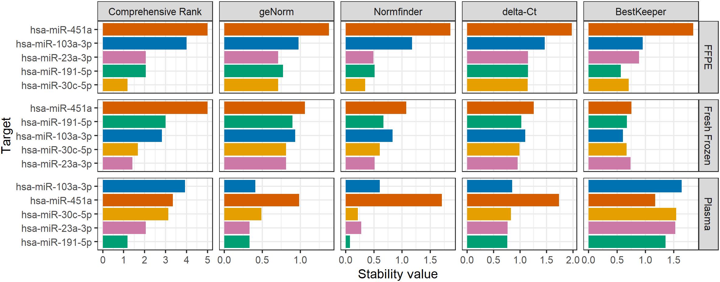
Figure 6. Example output of the colored .png file created with the rs_graph functionOnce the graph has the desired appearance, it can be exported to a number of different image file types. Again, type help(rs_graph) to see a comprehensive list of argument options. Here, we will create the default graph with the colors that were selected previously. To create the image file, a filename should be passed to the function:
rs_graph(results, filename= "Ovarian Cancer", colors = colors)
Also here, the function will output width and height as well as a confirmation that a file was created and a file path:
> width set to 2400
> height set to 960
> A png file was created at: <PATH\TO\FILE\>
Inspect the image file that was created (Figure 6). If needed, adjust the size using the width and height given in the previous output as a reference. Resolution can be set using the res-parameter; smaller numbers will make lines and text smaller and finer:
rs_graph(results, filename = "Ovarian Cancer", colors = colors, width = 2000, res = 200)
Table export
Creating a table output can be useful in many ways:
• To store results in universal lightweight file formats like .csv or .tsv.
• To share via Excel or OpenDocument Spreadsheet.
• To present findings in a word file or in a publication. Here, we will create an Excel file (see Figure 5) as well as a docx-combi table (see Table 1) for each dataset.
Creating an Excel file: the default table type is .xlsx, so this does not need to be specified:
rs_exporttable(results, filename = "Ovarian Cancer")
In this case, three .xlsx-files are created, one for each dataset.
Creating a docx-combi type table can be done by setting the tabletype parameter:
rs_exporttable(results, filename = "Ovarian Cancer", tabletype = "docx-combi")
Running individual algorithms
Stability values from each algorithm can be obtained individually. In this case, datasets must be passed individually:
rs_genorm(inputData$Plasma)
rs_normfinder(inputData$Plasma)
rs_deltact(inputData$Plasma)
rs_bestkeeper(inputData$Plasma)
Normfinder ungrouped and grouped stability analysis and paired candidate stability
Since it is recommended to use more than one reference gene, it may be of interest to identify pairs of targets, which are most stable in combination. If a set of reference targets have been chosen, these can be crudely validated through the Normfinder algorithm, which is able to provide further stability statistics and assessment of stability between groups and of pairs of genes. This approach is beneficial for identifying stable pairs and to compare selected references.
In the following example, we will use the Normfinder algorithm as a quick check of the selected references selected previously for fresh frozen and FFPE tissues.
Perform individual Normfinder analysis on Fresh frozen and FFPE datasets.
rs_normfinderFull(inputData$Fresh_Frozen, Groups = FALSE)
Giving the output:
$Ordered GroupSD hsa-miR-23a-3p 0.512 hsa-miR-30c-5p 0.607 hsa-miR-191-5p 0.668 hsa-miR-103a-3p 0.830 hsa-miR-451a 1.075 $PairOfGenes Gene1 Gene2 GroupSD 1 hsa-miR-30c-5p hsa-miR-23a-3p 0.424 This output indicates that, for the fresh frozen samples, a combination of hsa-miR-30c-5p and hsa-miR-23a-3p are the most stable pair. This is in agreement with the previous results that showed that hsa-miR-23a-3p and hsa-miR-30c-3p were the two most stable targets.
rs_normfinderFull(inputData$FFPE, Groups = FALSE)
Giving the output:
$Ordered GroupSD hsa-miR-30c-5p 0.344 hsa-miR-23a-3p 0.493 hsa-miR-191-5p 0.513 hsa-miR-103a-3p 1.179 hsa-miR-451a 1.857 This output indicates that, for the FFPE samples, hsa-miR-30c-5p and hsa-miR-23a-3p are the most stable. This is in agreement with the previous Normfinder results.
Note: Since no PairOfGenes are shown, no candidates were assessed as stable enough in a first round of calculations for paired analysis. This threshold is by default set to 0.25; however, it can be set via the pStabLim argument.
If differential expression is to be evaluated between two sample types, for example before or after treatment, it may be of interest to find target references that in combination show high stability between the two sample types. Here, we will use the Normfinder grouped analysis to identify stable pairs of references candidates for comparing expression across fresh frozen and FFPE tissue.
Perform a full Normfinder grouped analysis on the Fresh frozen and FFPE datasets.
First, we need to create a grouped dataset.
freshFrozen <- inputData$Fresh_Frozen
freshFrozen$group <- 1
FFPE <- inputData$FFPE
FFPE$group <- 2
Grouped <- rbind(freshFrozen, FFPE)
Now, perform the analysis:
rs_normfinderFull(Grouped, Groups = TRUE)$ PairOfGenes
Note: Here, we only select the PairOfGenes table to be printed.
Giving the output:
Gene1 Gene2 Stability 1 hsa-miR-30c-5p hsa-miR-103a-3p 0.128 2 hsa-miR-30c-5p hsa-miR-191-5p 0.086 3 hsa-miR-30c-5p hsa-miR-23a-3p 0.079 4 hsa-miR-103a-3p hsa-miR-191-5p 0.133 5 hsa-miR-103a-3p hsa-miR-23a-3p 0.127 6 hsa-miR-191-5p hsa-miR-23a-3p 0.088 According to Normfinder grouped analysis, hsa-miR-30c-5p and hsa-miR-191-5p are deemed the most stable pair across two groups.
Data analysis
Conclusions
In this protocol, we show how to perform stability analysis using widely used algorithms: geNorm, Normfinder, delta-Ct, BestKeeper, and RefFinder by the RefSeeker package for R. This protocol is easy to follow with its step-by-step guide and allows non-R programmers to perform stability analyses. It can be used to identify stable references in any kind of expression analysis and gives great options for data export of ready-to-publish graphs and tables.
Validation of protocol
This protocol or parts of it has been used and validated in the following research article:
Lopacinska-Jørgensen et al. (2023). Strategies for data normalization and missing data imputation and consequences for potential diagnostic microRNA biomarkers in epithelial ovarian cancer cancer. PLoS One (Table 3, Table 5 and Table S3).
Acknowledgments
We thank Douglas Vinicius Oliveira for valuable discussions. Also, we thank Rasmus Adalbert Meldgaard for early testing of the package. We are grateful to the Danish CancerBiobank (Bio- and GenomeBank Denmark) and the Danish Gynecologic Cancer Database for making specimens and data available for use in the present study. This work was founded by: The Mermaid Foundation, URL: http://www.mermaidprojektet.dk/ (PHDP, JLJ, CKH, and EVH received the funding), Danish Cancer Research Foundation: URL:http://www.dansk-kraeftforsknings-fond.dk/ (EVH received the funding), and Herlev Hospital Research Council, URL: https://www.herlevhospital.dk/forskning/ (EVH received the funding).
Competing interests
The authors declare no competing interests.
References
- Andersen, C. L., Jensen, J. L. and Ørntoft, T. F. (2004). Normalization of Real-Time Quantitative Reverse Transcription-PCR Data: A Model-Based Variance Estimation Approach to Identify Genes Suited for Normalization, Applied to Bladder and Colon Cancer Data Sets. Cancer Res. 64(15): 5245–5250.
- Bustin, S. A., Benes, V., Garson, J. A., Hellemans, J., Huggett, J., Kubista, M., Mueller, R., Nolan, T., Pfaffl, M. W., Shipley, G. L., et al. (2009). The MIQE Guidelines: Minimum Information for Publication of Quantitative Real-Time PCR Experiments. Clin. Chem. 55(4): 611–622.
- De Spiegelaere, W., Dern-Wieloch, J., Weigel, R., Schumacher, V., Schorle, H., Nettersheim, D., Bergmann, M., Brehm, R., Kliesch, S., Vandekerckhove, L., et al. (2015). Reference Gene Validation for RT-qPCR, a Note on Different Available Software Packages. PLoS One 10(3): e0122515.
- Faraldi, M., Gomarasca, M., Sansoni, V., Perego, S., Banfi, G. and Lombardi, G. (2019). Normalization strategies differently affect circulating miRNA profile associated with the training status. Sci. Rep. 9(1): e1038/s41598-019-38505-x.
- Petersen, P. H. D., Lopacinska-Jørgensen, J., Oliveira, D. V. N. P., Høgdall, C. K. and Høgdall, E. V. (2022). miRNA Expression in Ovarian Cancer in Fresh Frozen, Formalin-fixed Paraffin-embedded and Plasma Samples. In Vivo 36(4): 1591–1602.
- Pfaffl, M. W., Tichopad, A., Prgomet, C. and Neuvians, T. P. (2004). Determination of stable housekeeping genes, differentially regulated target genes and sample integrity: BestKeeper – Excel-based tool using pair-wise correlations. Biotechnol. Lett 26(6): 509–515.
- R Core Team. (2022). R: A language and environment for statistical computing 2022.
- Silver, N., Best, S., Jiang, J. and Thein, S. L. (2006). Selection of housekeeping genes for gene expression studies in human reticulocytes using real-time PCR. BMC Mol. Biol. 7(1): e1186/1471-2199-7-33.
- Sundaram, V. K., Sampathkumar, N. K., Massaad, C. and Grenier, J. (2019). Optimal use of statistical methods to validate reference gene stability in longitudinal studies. PLoS One 14(7): e0219440.
- Vandesompele, J., De Preter, K., Pattyn, F., Poppe, B., Van Roy, N., De Paepe, A., and Speleman, F. (2002) Accurate normalization of real-time quantitative RT-PCR data by geometric averaging of multiple internal control genes. Genome Biol. 3: research0034.1.
- Xie, F., Xiao, P., Chen, D., Xu, L. and Zhang, B. (2022). RefFinder. Accessed February 21, 2022.
- Xie, F., Xiao, P., Chen, D., Xu, L. and Zhang, B. (2012). miRDeepFinder: a miRNA analysis tool for deep sequencing of plant small RNAs. Plant Mol. Biol. 80(1): 75–84.
Supplementary information
The following supporting information can be downloaded here:
File S1. Example of a rs_reffinder result output.
Article Information
Publication history
Published: Sep 5, 2023
Copyright
© 2023 The Author(s); This is an open access article under the CC BY-NC license (https://creativecommons.org/licenses/by-nc/4.0/).
How to cite
Dalsbo Petersen, P. H., Lopacinska-Joergensen, J., Høgdall, C. K. and Høgdall, E. V. (2023). Expression Stability Analysis of Candidate References for Normalization of RT-qPCR Data Using RefSeeker R package. Bio-protocol 13(17): e4801. DOI: 10.21769/BioProtoc.4801.
Category
Molecular Biology > RNA > qRT-PCR
Bioinformatics and Computational Biology
Do you have any questions about this protocol?
Post your question to gather feedback from the community. We will also invite the authors of this article to respond.
![]() Tips for asking effective questions
Tips for asking effective questions
+ Description
Write a detailed description. Include all information that will help others answer your question including experimental processes, conditions, and relevant images.