
- Submit a Protocol
- Receive Our Alerts
- EN

- Protocols

- Articles and Issues
- For Authors
- About
- Become a Reviewer

Controlled Level of Contamination Coupled to Deep Sequencing (CoLoC-seq) Probes the Global Localisation Topology of Organelle Transcriptomes
Published: Vol 13, Iss 18, Sep 20, 2023 DOI: 10.21769/BioProtoc.4820 Views: 271
Reviewed by: Alessandro DidonnaMarina Sánchez PetidierRajesh D Gunage
Original research article
The authors used this protocol in:
Dec 2022

Protocol Collections
Comprehensive collections of detailed, peer-reviewed protocols focusing on specific topics


Abstract
Information on RNA localisation is essential for understanding physiological and pathological processes, such as gene expression, cell reprogramming, host–pathogen interactions, and signalling pathways involving RNA transactions at the level of membrane-less or membrane-bounded organelles and extracellular vesicles. In many cases, it is important to assess the topology of RNA localisation, i.e., to distinguish the transcripts encapsulated within an organelle of interest from those merely attached to its surface. This allows establishing which RNAs can, in principle, engage in local molecular interactions and which are prevented from interacting by membranes or other physical barriers. The most widely used techniques interrogating RNA localisation topology are based on the treatment of isolated organelles with RNases with subsequent identification of the surviving transcripts by northern blotting, qRT-PCR, or RNA-seq. However, this approach produces incoherent results and many false positives. Here, we describe Controlled Level of Contamination coupled to deep sequencing (CoLoC-seq), a more refined subcellular transcriptomics approach that overcomes these pitfalls. CoLoC-seq starts by the purification of organelles of interest. They are then either left intact or lysed and subjected to a gradient of RNase concentrations to produce unique RNA degradation dynamics profiles, which can be monitored by northern blotting or RNA-seq. Through straightforward mathematical modelling, CoLoC-seq distinguishes true membrane-enveloped transcripts from degradable and non-degradable contaminants of any abundance. The method has been implemented in the mitochondria of HEK293 cells, where it outperformed alternative subcellular transcriptomics approaches. It is applicable to other membrane-bounded organelles, e.g., plastids, single-membrane organelles of the vesicular system, extracellular vesicles, or viral particles.
Key features
• Tested on human mitochondria; potentially applicable to cell cultures, non-model organisms, extracellular vesicles, enveloped viruses, tissues; does not require genetic manipulations or highly pure organelles.
• In the case of human cells, the required amount of starting material is ~2,500 cm2 of 80% confluent cells (or ~3 × 10⁸ HEK293 cells).
• CoLoC-seq implements a special RNA-seq strategy to selectively capture intact transcripts, which requires RNases generating 5′-hydroxyl and 2′/3′-phosphate termini (e.g., RNase A, RNase I).
• Relies on nonlinear regression software with customisable exponential functions.
Graphical overview
Background
Knowing the localisation topology of transcripts with respect to organelle membranes (inside vs. outside) is critical for the understanding of RNA transactions in various subcellular locations. Selective RNA packaging into viral particles, extracellular vesicles, and ribonucleoproteins (RNPs) attracted much attention over the last two decades (Bresnahan and Shenk, 2000; K. Wang et al., 2010; Arroyo et al., 2011; Routh et al., 2012; Jeppesen et al., 2019; Murillo et al., 2019; Lécrivain and Beckmann, 2020; Gruner and McManus, 2021). Even more intriguing are the intricate interactions between the genetic systems of the nucleus, mitochondria, and plastids inside eukaryotic cells (Woodson and Chory, 2008; L. Levin et al., 2014; Quirós et al., 2016). These organelles possess their own genomes and locally produced transcriptomes. However, in many species, select nuclear-encoded RNAs (primarily tRNAs) enter mitochondria to participate in translation, blurring borders between transcriptomes (Schneider, 2011; Sieber et al., 2011; Jeandard et al., 2019). The scope of such RNA relocation pathways remains insufficiently understood. Therefore, robust genome-wide approaches are required to obtain comprehensive and reliable local transcriptomes.
Confident assignment of RNA localisation topology is challenging, and many approaches have been proposed (Jeandard et al., 2019). In fractionation-based techniques, organelles of interest are purified and treated with a non-specific RNase to degrade contaminant transcripts sticking to their surface. The remaining RNAs, detected by northern blotting, RT-PCR, or RNA-seq, are considered as residing inside the organelles. Although this strategy remains most widely used due to its simplicity and applicability to virtually any species, including non-model, genetically intractable organisms, cell cultures, and tissues (Mercer et al., 2011; Geiger and Dalgaard, 2017), its simple experimental setup turned out to be over-optimistic: some short, structured transcripts embedded in stable RNPs resist degradation, leading to prohibitively high false-positive rates. This caveat is mostly resolved by proximity labelling approaches that use organelle-restricted biochemical tagging of RNA molecules in situ to enable their selective enrichment and identification (Kaewsapsak et al., 2017; Fazal et al., 2019; P. Wang et al., 2019; Zhou et al., 2019; Medina-Munoz et al., 2020; Engel et al., 2021). However, these methods are usually biased against shorter, non-polyadenylated, and lowly abundant transcripts, and require genetic introduction of engineered tagging enzymes targeted to the organelle of interest, which limits their application to model species with tractable genomes and well-characterised protein localisation pathways.
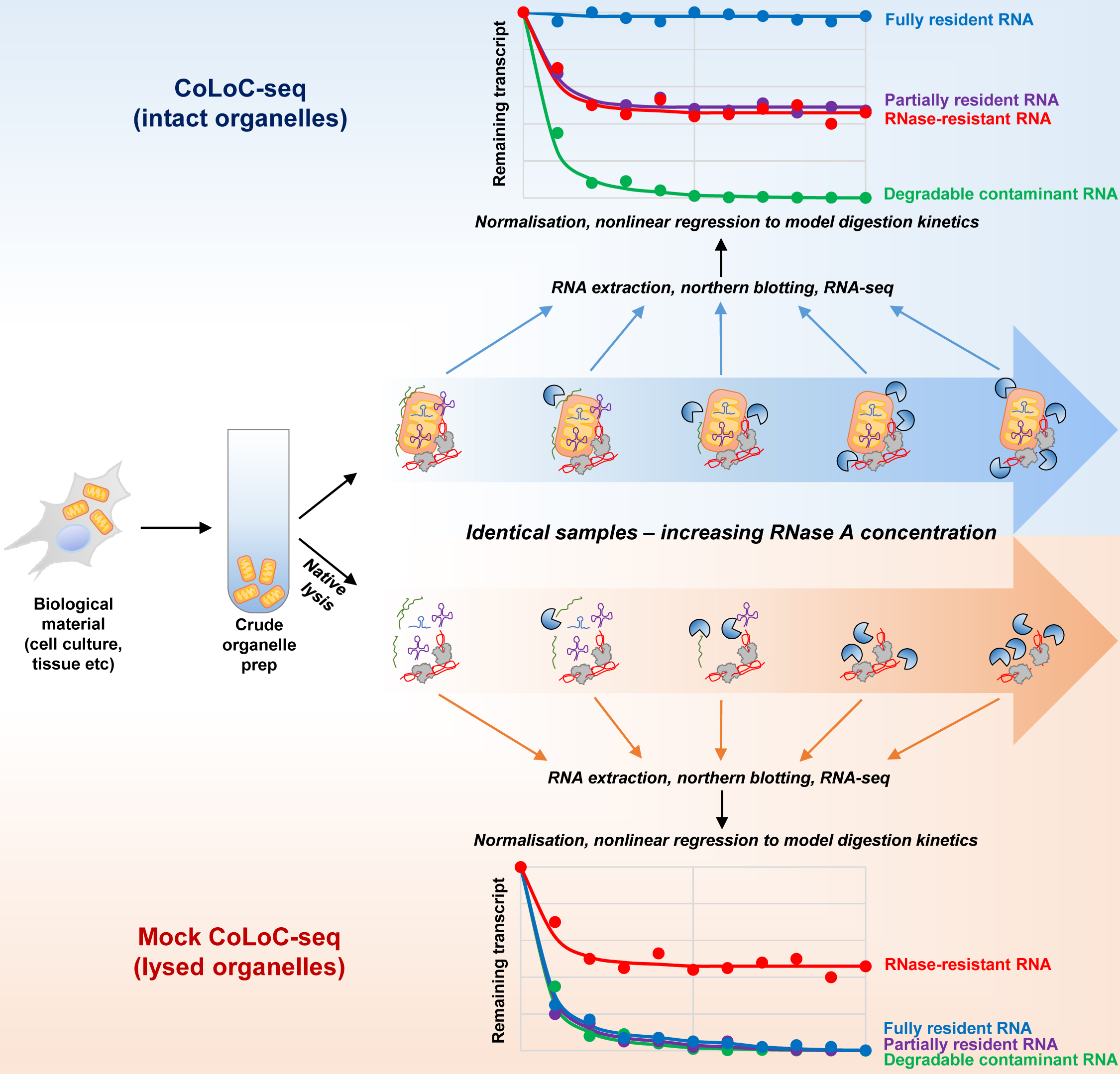
Here, we describe Controlled Level of Contamination coupled to deep sequencing (CoLoC-seq), which marries the accessibility and generality of fractionation-based approaches with the selectivity and robustness of proximity labelling techniques (Jeandard et al., 2023). In a standard CoLoC-seq pipeline (Figure 1, the blue branch), a preparation of intact organelles of interest is split into a suite of samples subjected to a gradient of RNase concentrations. This creates transcript-specific digestion kinetics, amenable to straightforward mathematical modelling, which tells whether a certain RNA fully partakes in the reaction (as expected for contaminants) or if there is a pool of unavailable molecules protected from the RNase. In a parallel Mock CoLoC-seq experiment (Figure 1, the orange branch), the same organelles are first mildly lysed with a detergent to solubilise membranes and then split in a series of identical samples for RNase treatment. Therefore, by measuring the same digestion kinetics in the mildly lysed organelles, one can determine whether the RNA protection is conferred by the organellar membranes or by unrelated factors, such as proteins or intricate structures (such unreactive RNAs are likely false positives).
Successfully tested on human mitochondria, CoLoC-seq outperformed other fractionation-based and proximity labelling approaches, especially in assigning the localisation topology of shorter non-coding RNAs. It can be applied to any RNase-impermeable entity, including eukaryotic organelles, endosymbionts, enveloped and some non-enveloped viruses, and extracellular vesicles.
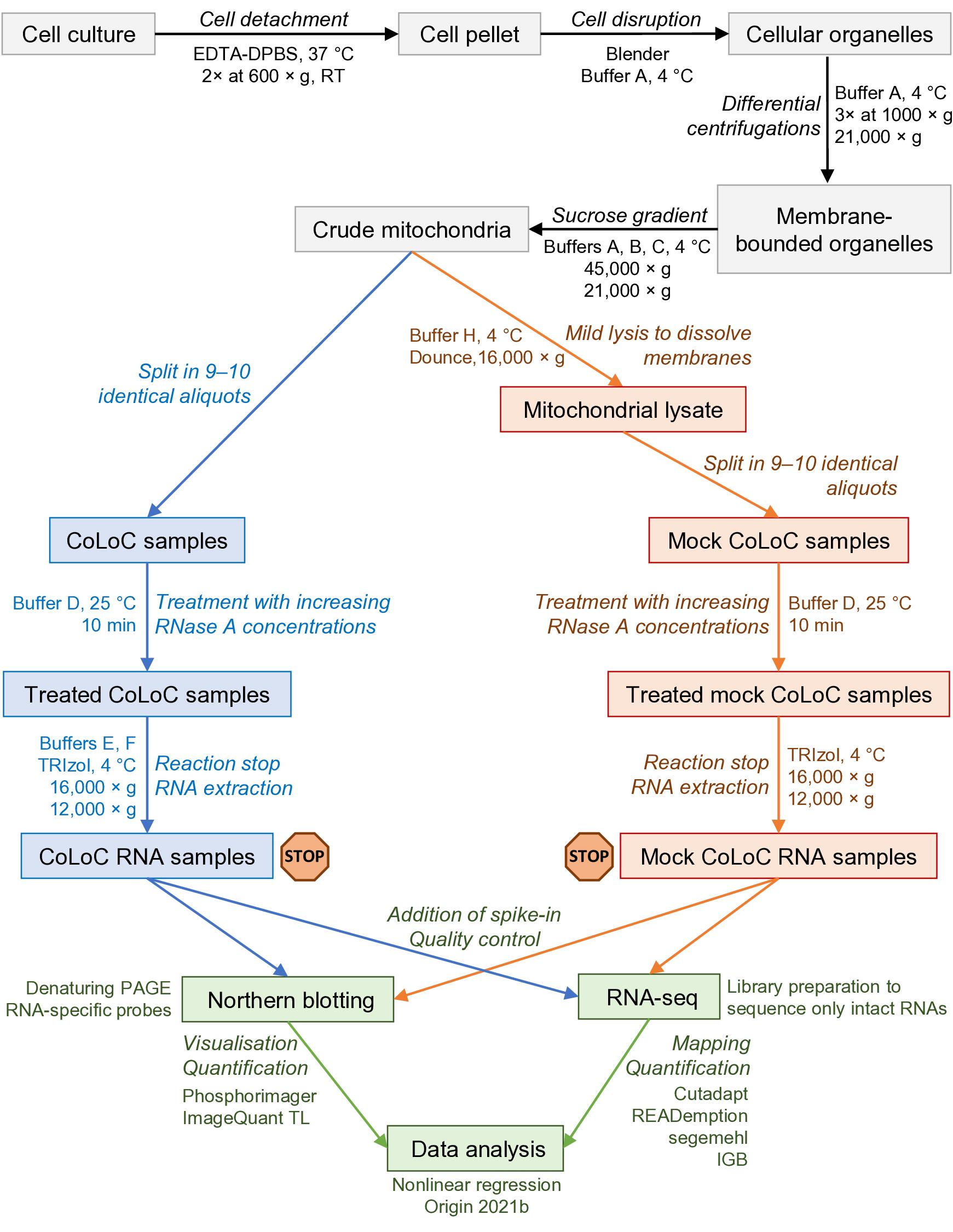
Figure 1. Overview of the protocol and its main steps. The part in grey covers the isolation of crude mitochondria, blue and orange correspond to the CoLoC and Mock CoLoC procedures, respectively, and green is data acquisition and analysis. The stop signs show the steps where the protocol can be safely interrupted without compromising the outcome of the experiment.
Materials and reagents
Biological materials
The CoLoC-seq was performed on mitochondria isolated from the human Flp-In T-REx 293 cells (Thermo Fisher Scientific, catalog number: R78007). One complete set of CoLoC-seq and Mock CoLoC-seq samples requires approximately 2,500 cm2 of nearly confluent cells (equivalent to ~3 × 10⁸ HEK293 cells) devoid of mycoplasma contamination. For application of CoLoC-seq to other systems and cellular compartments, the optimal amount of starting material should be determined empirically.
Reagents
EDTA (Sigma-Aldrich, catalog number: E4884)
Tris base (Sigma-Aldrich, catalog number: 11814273001)
Sucrose (Sigma-Aldrich, catalog number: S0389)
Sorbitol (Sigma-Aldrich, catalog number: S1876)
NaCl (Sigma-Aldrich, catalog number: S9888)
Bovine serum albumin, lyophilized, fatty acid free (Euromedex, catalog number: 1035-70-C)
NaOH (Sigma-Aldrich, catalog number: 655104)
Bromophenol blue (Sigma-Aldrich, catalog number: B0126)
Deionised formamide (Sigma-Aldrich, catalog number: S4117)
Dulbecco’s phosphate buffered saline (DPBS 1×) (Sigma-Aldrich, catalog number: D5773)
20% sodium dodecyl sulfate (SDS) (Euromedex, catalog number: EU-0660-B)
n-dodecyl-β-D-maltoside (Sigma-Aldrich, catalog number: D4641); store at -20 °C
Glycogen (Sigma-Aldrich, catalog number: G8876); store at 4 °C
TBE 10× (Euromedex, catalog number: ET020-C)
Urea (Sigma-Aldrich, catalog number U5378)
40% acrylamide/bis-acrylamide (19:1) (Carl Roth, catalog number: A516.1); store at 4 °C
Ammonium persulfate (Euromedex, catalog number: EU0009-B)
N,N,N’,N’-Tetramethyl ethylenediamine (TEMED) (Euromedex, catalog number: 50406)
Ethidium bromide 1% (Biosolve BV, catalog number: 05412341); store at 4 °C
SSC buffer 20× (Euromedex, catalog number: BI-D0623-1L)
Denhardt’s solution 50× (Thermo Fisher Scientific, catalog number: 750018); store at -20 °C
TE (Tris-EDTA buffer), pH 7.4 (10×) (Euromedex, catalog number: BI-USD8211-1L)
DNase I (Thermo Fisher Scientific, catalog number: EN0525); store at -20 °C
RNase A, DNase- and protease-free, 10 mg/mL (Thermo Fisher Scientific, catalog number: EN0531); store at -20 °C
SUPERase In RNase inhibitor (Thermo Fisher Scientific, catalog number: AM2694); store at -20 °C
AMPure XP kit (Beckman Coulter, catalog number: A63881)
Bradford assay ROTI Nanoquant (Carl Roth, catalog number: K880.1); store at 4 °C
TRIzol reagent (Thermo Fisher Scientific, catalog number: 15596026); store at 4 °C
γ-[32P]-ATP (10 Ci/L, 3,000 Ci/mmol) (PerkinElmer, catalog number: BLU002A100UC). Should be used within approximately one month (32P half-life is 14.268 days); store at -20 °C
Polynucleotide kinase (PNK) and 10× kinase reaction buffer A (Promega, catalog number: M4101); store at -20 °C
Chloroform (Carl Roth, catalog number: 6340.4)
Isopropanol (Carl Roth, catalog number: CP41.1)
Ethanol (Dutscher, Carlo Erba, catalog number: 3086072-CER)
Solutions
Sterile 0.1 M EDTA (see Recipes)
Sterile EDTA-DPBS (see Recipes)
Tris-HCl 0.1 M, pH 6.7 (see Recipes)
Sucrose 3.3 M (see Recipes)
Sorbitol 3 M (see Recipes)
NaCl 1 M (see Recipes)
NaOH 6% (see Recipes)
Buffer A (see Recipes)
Buffer B (see Recipes)
Buffer C (see Recipes)
Buffer D (see Recipes)
Buffer E (see Recipes)
Buffer F (see Recipes)
Buffer H (see Recipes)
RNA loading buffer (see Recipes)
RNA denaturing polyacrylamide gel (see Recipes)
Ammonium persulfate 10% (see Recipes)
Pre-hybridisation buffer (see Recipes)
Hybridisation buffer (see Recipes)
Washing buffer (see Recipes)
Stripping buffer (see Recipes)
Ethanol 80% (see Recipes)
RNase A dilutions in buffer D (see Recipes)
Glycogen 20 μg/μL (see Recipes)
Ethidium bromide 0.0001% (see Recipes)
Recipes
Sterile 0.1 M EDTA (store at 4 °C)
Stir 37.2 g of EDTA in 800 mL of H2O. Add NaOH to adjust pH to 8. Dilute the solution to 1 L with water. Filter solution through a 0.22 μm filter.
Reagent Final concentration Quantity EDTA 0.1 M 37.2 g H2O n/a n/a NaOH n/a n/a Total n/a 1,000 mL Sterile EDTA-DPBS (store at room temperature)
Reagent Final concentration Quantity DPBS (1×) 1× 9.6 g EDTA (0.1 M) 2.5 mM 25 mL H2O n/a 975 mL Total n/a 1,000 mL Tris-HCl 0.1 M, pH 6.7 (store at room temperature)
Stir 12.11 g of Tris base in 800 mL of H2O. Add concentrated HCl under the fume hood to adjust pH to 6.7. Dilute the solution to 1 L with water.
Reagent Final concentration Quantity Tris base 0.1 M 12.11 g HCl (concentrated) n/a n/a H2O n/a n/a Total n/a 1,000 mL Sucrose 3.3 M (store at 4 °C)
Reagent Final concentration Quantity Sucrose 3.3 M 112.86 g H2O n/a n/a Total n/a 100 mL Sorbitol 3 M (sterilise by short autoclaving; store at 4 °C)
Reagent Final concentration Quantity Sorbitol 3 M 54.65 g H2O n/a n/a Total n/a 100 mL NaCl 1 M (store at room temperature)
Reagent Final concentration Quantity NaCl 1 M 5.84 g H2O n/a n/a Total n/a 100 mL NaOH 6% (store at room temperature)
Reagent Final concentration Quantity NaOH 6% 0.6 g H2O n/a 10 mL Total n/a 10 mL Buffer A (store at 4 °C)
Reagent Final concentration Quantity Sorbitol (3 M) 0.6 M 20 mL Tris-HCl (0.1 M, pH 6.7) 10 mM 10 mL H2O n/a 70 mL Total n/a 100 mL Buffer B (store at 4 °C)
Reagent Final concentration Quantity Sucrose (3.3 M) 1.65 M 50 mL Tris-HCl (0.1 M, pH 6.7) 10 mM 10 mL H2O n/a 40 mL Total n/a 100 mL Buffer C (store at 4 °C)
Reagent Final concentration Quantity Sucrose (3.3 M) 0.6 M 18 mL Tris-HCl (0.1 M, pH 6.7) 10 mM 10 mL H2O n/a 72 mL Total n/a 100 mL Buffer D (store at 4 °C)
Reagent Final concentration Quantity Sorbitol (3 M) 0.6 M 20 mL NaCl (1 M) 200 mM 20 mL EDTA (0.1 M) 2 mM 2 mL Tris-HCl (0.1 M, pH 6.7) 10 mM 10 mL H2O n/a 48 mL Total n/a 100 mL Buffer E (store at 4 °C)
Reagent Final concentration Quantity Sorbitol (3 M) 0.6 M 20 mL EDTA (0.1 M) 5 mM 5 mL Tris-HCl (0.1 M, pH 6.7) 10 mM 10 mL H2O n/a 65 mL Total n/a 100 mL Buffer F (store at 4 °C)
Reagent Final concentration Quantity Sorbitol (3 M) 0.6 M 20 mL EDTA (0.1 M) 1 mM 1 mL Tris-HCl (0.1 M, pH 6.7) 10 mM 10 mL H2O n/a 69 mL Total n/a 100 mL Buffer H (store at 4 °C)
Reagent Final concentration Quantity Sorbitol (3 M) 0.6 M 0.2 mL n-dodecyl-β-D-maltoside 1% 10 mg Tris-HCl (0.1 M, pH 6.7) 10 mM 0.1 mL H2O n/a 0.7 mL Total n/a 1 mL RNA loading buffer
Prepare on RNase-free water and add a few crystals of bromophenol blue until the solution has a deep colour but is still transparent; store at -20 °C in 1 mL aliquots.
Reagent Final concentration Quantity SDS (20%) 0.025% 0.0125 mL EDTA (0.1 M) 18 mM 1.8 mL Deionised formamide n/a 8.1875 mL Total n/a 10 mL RNA denaturing polyacrylamide gel
Prepare on RNase-free water. Store at 4 °C and pre-warm before use if urea precipitates.
Reagent Final concentration Quantity TBE 10× 1× 10 mL Urea 8 M 48 g 40% acrylamide/bis-acrylamide (19:1) 6% 15 mL H2O n/a n/a Total n/a 100 mL Ammonium persulfate 10% (store at 4 °C for one month)
Reagent Final concentration Quantity Ammonium persulfate 10% 10 g H2O n/a n/a Total n/a 100 mL Pre-hybridisation buffer (store at room temperature)
Reagent Final concentration Quantity SSC 20× 6× 300 mL Denhardt’s solution 50× 5× 100 mL SDS (20%) 0.2% 10 mL H2O n/a 590 mL Total n/a 1,000 mL Hybridisation buffer (prepare immediately before use)
Reagent Final concentration Quantity Pre-hybridisation buffer 1× 0.45× 9 mL TE 10× 0.5× 1 mL NaCl (1 M) 0.5 M 10 mL Total n/a 20 mL Washing buffer (store at room temperature)
Reagent Final concentration Quantity SSC 20× 5× 250 mL SDS (20%) 0.1% 5 mL H2O n/a 745 mL Total n/a 1,000 mL Stripping buffer (store at room temperature)
Reagent Final concentration Quantity SSC 20× 0.01× 0.5 mL SDS (20%) 0.1% 5 mL H2O n/a 994.5 mL Total n/a 1,000 mL Ethanol 80%
Reagent Final concentration Quantity Ethanol (100%) 80% 800 mL H2O 20% 200 mL Total n/a 1,000 mL RNase A dilutions in buffer D (final volume 200 μL; prepare immediately before use and keep on ice)
To prepare the working RNase A solution at 10 μg/mL, dilute 2 μL of RNase A (10 mg/mL) in 1,998 μL of buffer D and mix well.
Reagent Final concentration Quantity Buffer D volume RNase A working solution (10 μg/mL)
0.1 μg/mL
0.2 μg/mL
0.6 μg/mL
1.2 μg/mL
2.0 μg/mL
2.6 μg/mL
3.2 μg/mL
4.0 μg/mL
6.0 μg/mL
2 μL
4 μL
12 μL
24 μL
40 μL
52 μL
64 μL
80 μL
120 μL
198 μL
196 μL
188 μL
176 μL
160 μL
148 μL
136 μL
120 μL
80 μL
Glycogen 20 μg/μL (aliquot and store at -20 °C)
Reagent Final concentration Quantity Glycogen 20 μg/μL 200 mg H2O n/a 10 mL Total n/a 10 mL Ethidium bromide 0.0001% prepared on RNase-free water (store at 4 °C)
Reagent Final concentration Quantity Ethidium bromide 1% 0.0001% 10 μL RNase-free water n/a 100 mL Total n/a 100 mL
Laboratory supplies
Stericup Quick Release-GV sterile vacuum filtration system 0.22 µm pore size (Merck, catalog number: S2GVU10RE)
Yeast tRNA-derived spike-in transcript, which does not cross-map to the human genome, to enable data normalization:
5′-GAGAAGUAAGCACUGUAAAGGUUUUAGAGCUAGAAAUAGCAAGUUAAAAUAAGGCUAGUCCGUUAUCAACUUGAAAAAGUGGCACCGAGUCGGUGCUUGCCUUGUUGGCGCAAUCGGUAGCGCGUAUGACUCUUAAUCAUAAGGUUAGGGGUUCGAGCCCCCUACAGGGCUCCA-3′
Note: Depending on biological material, compatible spike-in transcript(s) should be used, with a sequence that does not cross-map with the genome of the examined organism. A spike-in transcript can be purchased or synthesised by in vitro T7 transcription (as in this case).
Amersham Hybond-N+ membrane optimised for nucleic acid transfer (Cytiva, catalog number: RPN203B)
Single-use spectrophotometer cuvette 1.6 mL Semi-micro type ClearLine (Dutscher, catalog number: 030101)
Micro Bio-Spin P-6 chromatography columns (Bio-Rad, catalog number: 7326200)
Custom DNA oligonucleotide probes for northern blot hybridisation. The oligonucleotides used for CoLoC-seq of human mitochondria are listed in Jeandard et al. (2023), Table S1.
Equipment
Micropipette PIPETMAN P2, 0.2–2 μL (Gilson, catalog number: F144054M)
Micropipette PIPETMAN P20, 2–20 μL (Gilson, catalog number: F144056M)
Micropipette PIPETMAN P200, 20–200 μL (Gilson, catalog number: F144058M)
Micropipette PIPETMAN P1000, 100–1,000 μL (Gilson, catalog number: F144059M)
Vacuum aspiration system (Integra Bioscience VACUSAFE Aspiration System, Fisher Scientific, catalog number: 11636620)
Refrigerated tabletop centrifuge for 50 mL tubes (Eppendorf 5810R, Eppendorf, catalog number: 5811000015)
Refrigerated tabletop centrifuge for 2 mL tubes (Eppendorf 5427R, Eppendorf, catalog number: 5409000010)
Refrigerated high-speed centrifuge (Avanti J-E, Beckman Coulter, catalog number: 369005) with a F0850 fixed-angle aluminium rotor (Beckman Coulter, catalog number: 364640)
Polycarbonate 50 mL bottles with screw cap for the F0850 rotor (Beckman Coulter, catalog number: 357002)
Waring two-speed blender (The Laboratory Store, catalog number: 8010EB)
Refrigerated ultracentrifuge Optima XPN-100 (Beckman Coulter, catalog number: A94469) with a swinging bucket SW 32 Ti (Beckman Coulter, catalog number: 369694)
Open-top thin-wall polypropylene tubes for a swinging bucket SW 32 Ti (Beckman Coulter, catalog number: 326823)
Water bath (e.g., VWR, catalog number: 76308-830)
Dounce homogenizer (VWR, catalog number: 432-0200)
Spectrophotometer (e.g., Eppendorf BioPhotometer 6131, Marshall Scientific, catalog number: E-BP6131)
Spectrophotometer NanoDrop (Thermo Fisher Scientific, NanoDrop 2000, catalog number: ND-2000)
Block heater (e.g., Stuart, DD Biolab, catalog number: 001150)
Gel electrophoresis chamber (e.g., BT Lab Systems, catalog number: BT206)
Low-current power supply (e.g., Consort EV233, Fisher Scientific, catalog number: 10369312)
Gel documentation system (e.g., E.A.S.Y. Doc Plus, Herolab, catalog number: 2809300)
Wet transfer tank (e.g., BT Lab Systems, catalog number: BT306)
High-current power supply (e.g., PowerPac HC, Bio-Rad, catalog number: 1645052)
UV lamp for RNA cross-linking (e.g., Hoefer UVC 500 Ultraviolet Crosslinker, Amersham Life Science, catalog number: 80-6222-50)
Rotating hybridisation oven (e.g., Problot 12 Hybridization Oven, Labnet, catalog number: H1200A-230V)
Plastic sealing machine (e.g., Manual heat sealer SK-SK 210 series, FALC Instruments, catalog number: 638.1430.20)
Phosphorimager plate (e.g., VWR, catalog number: 28-9564-75)
Exposition cassette (e.g., VWR, catalog number: 29-1755-23)
Light eraser for Phosphorimager plates (e.g., InmoClinc Screen X-ray film viewer, MedicalExpo, catalog number: 16300)
Phosphorimager scanner (e.g., GE Typhoon Trio Imager, GMI, SKU: 8149-30-0017)
Portable Geiger counter (e.g., Mini900 Ratemeter, Thermo Scientific, catalog number: MFG017)
Software and datasets
ImageQuant TL (v. 7.0, GE Healthcare)
Cutadapt (version 2.8) (available at https://pypi.org/project/cutadapt/2.8/)
READemption (version 0.4.3) (available at https://reademption.readthedocs.io/en/latest/)
Human genome sequence (Genome Reference Consortium Human Build 38 patch release 13)
READemption uses segemehl version 0.2.0-418 as the read aligner
Data analysis pipeline on Zenodo (https://doi.org/10.5281/zenodo.6389451)
Integrated Genome Browser (v. 9.1.8) (available at https://bioviz.org/)
Origin 2021b (v9.8.5.212, OriginLab Corporation) or similar nonlinear regression software
Procedure
Cell harvesting and crude fractionation
Human cell harvesting (here, we describe an example procedure for 2,500 cm2 of adherent HEK293 cells cultivated in eleven 225 cm2 flasks):
Gently aspirate the medium using a vacuum aspiration system. To each flask, add 25 mL of sterile EDTA-DPBS and incubate for 20 min at 37 °C.
Gently hit the flasks with a hand to facilitate cells detachment. Collect the cell suspension into six 50 mL tubes.
To collect the maximum of cells, rinse the flasks with 25 mL of EDTA-DPBS by transferring the solution from flask to flask. Divide the obtained cell suspension between the six half-filled 50 mL tubes from the previous step.
Pellet the cells by centrifugation at 600× g for 10 min at room temperature. Discard the supernatant.
Add 15 mL of sterile DPBS at room temperature to each tube and pool cell suspensions in two 50 mL tubes.
Pellet the cells by centrifugation at 600× g for 10 min at room temperature. Discard the supernatant.
Preparation of crude mitochondria (all procedures are carried out on ice with pre-chilled solutions and tubes):
Resuspend the cells in 30 mL of buffer A.
Disrupt the cells at high speed with a pre-chilled laboratory blender three times for 15 s, with 1 min intervals to prevent overheating. Place the homogenate into a 50 mL tube.
Remove cellular debris and nuclei by low-speed centrifugation in a refrigerated tabletop centrifuge at 1,000× g for 3 min at 4 °C. Transfer the supernatant into a new 50 mL tube.
Repeat the procedure described in A2c twice.
Note: The cell debris/nuclei pellet is easily dislodged and dispersed; one should pipette very carefully to limit this undesirable contamination.
Transfer the supernatant into polycarbonate 50 mL bottles with screw cap. Pellet crude mitochondria by centrifugation in a refrigerated high-speed centrifuge at 21,000× g for 30 min at 4 °C.
A brownish pellet will form. Carefully pipette the supernatant out.
Carefully but thoroughly resuspend the mitochondrial pellet in 8 mL of buffer A and split in four 2 mL portions.
Note: It is important to resuspend well the crude mitochondrial pellet and obtain a homogeneous suspension. However, do not overdo it to prevent the lysis of mitochondria.
Prepare four two-cushion sucrose gradients in SW 32 Ti centrifugation tubes. First, place 10 mL of buffer B in the tube. Then, carefully and slowly layer 15 mL of buffer C along the tube wall atop the first cushion using a soft, smoothly going pipette. Avoid disturbing the lower cushion.
Carefully load each 2 mL portion of crude mitochondria atop a two-cushion gradient.
Centrifuge in a refrigerated ultracentrifuge Optima XPN-100 with a swinging bucket SW 32 Ti rotor at 45,000× g for 1 h at 4 °C.
Collect the turbid mitochondria-containing interphase with a pipette.
Combine the interphases from the four tubes in a polycarbonate 50 mL bottle, dilute them with 30 mL of buffer A, and pellet the mitochondria again at 21,000× g for 30 min at 4 °C.
Carefully pipette out the supernatant.
Gently but thoroughly resuspend the mitochondrial pellet in 800 μL of buffer A. Critical: The suspension of mitochondria should be homogeneous. Save 500 μL of the suspension for a CoLoC-seq experiment (section B) and reserve the other 300 μL for a Mock CoLoC-seq experiment (section D). Keep them on ice.
CoLoC procedure
All procedures are carried out at 4 °C with pre-chilled solutions and tubes, unless specified differently; all centrifugations are performed in a refrigerated tabletop centrifuge for 2 mL tubes.
Measure protein concentration in the sample for the CoLoC-seq experiment by Bradford assay.
Note: The spectrophotometer should be calibrated for the Bradford assay, following the manufacturer’s instructions. To this end, one typically uses a series of bovine serum albumin solutions containing 1–10 μg of protein.
Dissolve 2 μL of the mitochondrial suspension in 40 μL of 6% NaOH. For the blank, use 2 μL of buffer A.
Add 760 μL of MilliQ water and mix thoroughly.
Add 200 μL of the Bradford solution, mix well, and transfer the suspension to a disposable plastic spectrophotometer cuvette.
After 60 s of incubation at room temperature, read the blank OD at 595 nm. Then read the mitochondrial protein sample OD at the same wavelength and determine its protein concentration using the standard curve. From 2,500 cm2 of nearly confluent HEK293 cells, one typically obtains 5–10 mg of crude mitochondria.
Adjust the mitochondrial suspension to 1.6 mg of protein per millilitre using buffer A.
Split the resulting suspension of mitochondria in a series of identical 80 μL samples. Ten samples must be sufficient to create an informative RNA depletion curve.
Prepare two series of 80 μL RNase A dilutions in buffer D with concentrations ranging from 0 to 6 μg/mL (e.g., 0, 0.1, 0.2, 0.6, 1.2, 2.0, 2.6, 3.2, 4.0, and 6.0 μg/mL). Use one series for the CoLoC and the other for the Mock CoLoC procedure.
Pre-warm the RNase A dilutions on water bath at 25 °C for 1 min.
Mix the 80 μL mitochondrial samples with the corresponding 80 μL RNase A dilutions and incubate on water bath at 25 °C for 10 min.
Dilute the reactions with ice-cold buffer E to 1.6 mL.
Centrifuge at 16,000× g for 20 min at 4 °C.
Resuspend the pellets thoroughly in 100 μL of buffer F.
RNA extraction
Caution: RNA extraction should be performed in a fume hood and with personal protection.
Add 1 mL of TRIzol and shake samples for 10 s (do not vortex). Pause point: Once TRIzol is added to the samples, they can be stored at -80 °C; otherwise, proceed to step C2.
Note: TRIzol is stored at 2–25 °C; however, it should be warmed up to room temperature before use.
Incubate samples for 5 min at room temperature.
Add 0.2 mL of chloroform and cap the tubes securely.
Shake the tubes vigorously by hand for 15 s.
Incubate for 3 min at room temperature.
Centrifuge the samples at 14,000× g for 15 min at 4 °C.
Carefully transfer the upper aqueous phase containing RNA to a new tube by angling the tube at ~45° and pipetting the solution out with a P200 micropipette. Critical: Take up the aqueous phase as completely as possible but avoid touching the protein-containing interphase. Contamination of RNA samples with protein may result in low-quality and/or artefactually degraded RNA.
Add 2 μL of 20 μg/μL glycogen to the samples to facilitate RNA precipitation.
Add 0.5 mL of isopropanol to the samples and mix thoroughly.
Let the RNA precipitate at -20 °C for 1 h. Pause point: The samples can be stored at -80 °C.
Centrifuge at 14,000× g for 20 min at 4 °C. Carefully decant the supernatant into a clean tube.
Note: RNA pellets sometimes do not stick well to the tube wall. Decanting the supernatant to another tube prevents the pellet loss; if needed, simply transfer the supernatant with the floating pellet back and repeat the centrifugation.
Wash the pellet with 0.5 mL of 80% ethanol.
Centrifuge at 14,000× g for 10 min at 4 °C. Decant the supernatant as previously.
Wash the pellet with 0.5 mL of 100% ethanol.
Centrifuge at 14,000× g for 10 min at 4 °C.
Decant the supernatant, as previously. Dry the pellets by leaving the tubes open on the bench for 5–10 min.
Fully dissolve RNA in 45 μL of RNase-free water. Pause point: Samples of isolated RNA can be stored at -80 °C.
Mix each sample of extracted RNA with 90 ng of a spike-in transcript to enable subsequent data normalization.
Add to each sample 5 μL of the 10× DNase I reaction buffer, 1 U of DNase I, and 20 U of SUPERase•In. Incubate for 30 min at 37 °C to digest residual DNA.
Re-extract RNA with TRIzol, as described in steps C1–C7. Precipitate it, as in steps C9–C16.
Note: No further glycogen addition is required, since the previously added glycogen partitions with RNA during extraction. Re-dissolve the RNA pellet in 20 μL of RNase-free water.
Measure RNA concentration in each sample with NanoDrop. Expected RNA concentrations are in the range of 50–200 ng/μL. Pause point: RNA samples can be stored at -80 °C.
Mock CoLoC procedure
Mix 300 μL of the reserved crude mitochondrial extract from step A2n with 300 μL of ice-cold buffer H.
Lyse the mitochondria on ice with 50 strokes in a small Dounce homogenizer.
Clear the lysate by centrifugation at 16,000× g for 20 min at 4 °C. Transfer the supernatant to a new tube.
Note: The remaining pellet must be relatively small, and the supernatant must be of yellow-to-brown colour, indicating good solubilisation of the mitochondrial contents. If the pellet is still big and the supernatant is colourless, repeat the lysis adding more buffer H.
Repeat step D3 to remove any remaining insoluble material.
Measure protein concentration in the cleared lysate by Bradford assay, as described in step B1.
Adjust the lysate to protein concentration of 1.6 mg/mL with ice-cold buffer A.
Split the resulting solution in a series of identical 80 μL samples in 2 mL tubes.
Perform RNase treatment in the same way as for the regular CoLoC procedure (steps B4–B6).
Centrifuge the reactions at 16,000× g for 40 min at 4 °C.
Add 1.44 mL of TRIzol. Pause point: The samples can be stored at -80 °C. Otherwise, proceed to step D11.
Incubate the samples at room temperature for 5 min. Add 320 μL of chloroform and extract RNA, as described in steps C4–C21.
Northern blotting
Caution: Work with radioactive material in a specially equipped lab using personal protection.
Note: While the northern blotting protocol described here is based on radioactive probes, viable non-radioactive alternatives also exist, e.g., irNorthern, using near-infrared fluorescence (Miller et al., 2018), and digoxigenin-labelled probes, exploiting western-like chemiluminescence detection (Höltke et al., 1992).
Take 1 μg of the 0 RNA sample (treated with 0 μg/mL RNase A). Take the same volume of all remaining samples in a series. (For example, if the 0 sample has the RNA concentration of 200 ng/μL, you should take 5 μL of each sample in this series, independently of the RNA concentration of the other samples.) (Note: RNA yield naturally decreases in samples treated with higher RNase A concentrations. Keeping the same volume fraction enables correct dosage for all samples of a series. Measuring the level of the spike-in RNA will further ensure equal sample loading.) Mix the RNA 1:1 (by volume) with RNA loading buffer. Caution: The RNA loading buffer contains formamide and should be manipulated under the hood.
Prepare a big (15–20 cm) and thick (1.5 mm) 6% RNA denaturing polyacrylamide gel by polymerising the gel solution by addition of 1/100 volume of 10% ammonium persulfate and 1/1,000 volume of TEMED.
Denature the samples at 95 °C for 5 min in a block heater.
Install the gel slot in the electrophoresis chamber and add a sufficient amount of 1× TBE buffer.
Just before loading the samples, thoroughly wash the pockets from urea 10 times by vigorous pipetting with a P1000 pipette.
Keep the samples on the bench for 1 min and load them immediately after the last wash of the pockets on the gel using a smoothly going pipette with a long thin tip.
Note: It is important to load the sample firmly and quickly on the very bottom of the well, avoiding spurts and bubbles.
Close the chamber and run the gel at 10 V/cm and 30 mA until bromophenol blue is approximately 3 cm from the bottom.
Carefully disassemble the sandwich. Stain the gel in 200 mL of 0.0001% ethidium bromide for 5 min. Visualise the ethidium fluorescence and record the resulting image with the help of a suitable UV-based gel documentation system.
Note: Minimise exposure of the gel to UV light to avoid RNA crosslinking.
Assemble a northern blot sandwich according to manufacturer’s instructions for a wet transfer tank. For example, use three sheets of Whatman paper with dimensions matching those of the gel. Moisten them with 0.5× TBE and apply them one upon the other, atop the sponge on the anode (+) side of the cassette. After each sheet, use a roller to gently chase air bubbles from the sandwich. Then, apply a Hybond-N+ membrane for nucleic acids transfer (moistened in 0.5× TBE) atop the Whatman sheets. Then, carefully place the gel on the membrane and cover it with three more moistened Whatman sheets. Close the sandwich.
Place the cassette in the corresponding wet transfer chamber filled with cold, freshly prepared TBE 0.5× buffer and perform transfer at 75 V and up to 3 A for 1.5 h in a cold room, with gentle magnet stirring.
Note: While 1.5 h is generally enough for a complete transfer, this step can be prolonged up to 3 h, at the experimenter’s convenience.
Disassemble the sandwich and air dry the membrane on a sheet of absorbing paper. Crosslink RNA to the membrane for 3 min in Hoefer UVC 500 Ultraviolet Crosslinker. Pause point: The dry membrane can be stored at 4 °C.
Place the membrane in a hybridisation glass tube, add 20 mL of pre-hybridisation buffer, and incubate in a slowly rotating hybridisation oven for 30 min at 65 °C. Make sure that the membrane is uniformly unfolded in the tube and does not fold back on itself (if this happens, simply invert the tube), and that all areas subject to hybridisation are in maximally identical conditions and uniformly covered with the liquid.
Replace the pre-hybridisation buffer with the hybridisation buffer and add 3–5 μL of the purified labelled probe.
Note: For 5′-[32P]-oligonucleotide labelling, see section F.
Incubate the membrane with the probe for at least 2 h (normally, over day or overnight) at 42 °C with continuous rotation in the hybridisation oven.
Note: If the probed transcript is of low abundance, the amount of the probe can be increased. If the probe is long or highly structured, it should be denatured and put on ice, as described in step F1, prior to its addition to hybridisation buffer. If the probe is very long (> 40 nt), it is recommended to increase the incubation temperature to 50–60 °C to avoid non-specific hybridisation. The optimal hybridisation temperature can be adjusted for each oligo individually, with 42 °C performing well for most probes.
To wash the blot, discard the hybridisation mix to a dedicated radioactive waste container, add 20 mL of the washing buffer, and rotate the tube in the hybridisation oven for 15 min at the same temperature. Caution: Do not discard radioactive solutions in the sink.
Discard the washing buffer in a dedicated radioactive waste container. Remove the membrane from the glass tube.
Dry the membrane on a sheet of absorbing paper on the bench. Seal it in a plastic film.
Expose the membrane overnight (or longer, up to a week, if the signal is expected to be weak) with a phosphorimager plate in an appropriate cassette. Shorter expositions are only needed if the signal is very strong (measurable with a portable counter) and becomes quickly saturated.
Scan the phosphorimager plate on Typhoon or a similar device using appropriate instrument settings.
Erase the residual signal from the plate with a light eraser.
Note: The phosphorimager plate bleaching is also recommended immediately before exposition (step E18) to reduce background.
To remove the previous probe for further hybridisations, rotate the membrane in a glass tube in the hybridisation oven in 20–30 mL of stripping buffer for 30 min at 63–65 °C. If the probe is very long and/or the signal is strong, remove it by rocking the membrane with an excess of stripping buffer in a water bath at 80 °C for 30 min. Then, proceed with the next hybridisation from step E13.
Oligonucleotide labelling
Caution: Work with radioactive material in a specially equipped lab using personal protection.
Prepare a 20 μL labelling reaction by mixing 13 μL of water, 1 μL of a 10 μM solution of the DNA oligonucleotide to label, 2 μL of 10× PNK buffer, 3 μL of [32P]-γ-ATP, and 1 μL of PNK.
Note: If the probed transcript is very abundant, one can take 1 μL of [32P]-γ-ATP and 15 μL of water instead (the rest of the mix will be the same). If the probe is very long (> 40 nt) or highly structured, mix 13 μL of water and 1 μL of a 10 μM solution of the DNA oligo and denature it at 95 °C for 1 min, then immediately put on ice for 1 min and quickly add the remaining components of the labelling mix, as described above. This usually increases labelling efficiency.
Incubate the reaction mixture at 37 °C for 30 min to 1 h. Caution: Shield the heating block with a Plexiglas screen to protect yourself and others from exposure to radioactivity.
Oligonucleotide purification:
Briefly vortex a Micro Bio-spin P-6 chromatography column.
Shake the drops down, break the bottom plug off, and insert the column in the corresponding collecting tube.
Open the upper lid, close it again to push air bubbles through, and open once again.
Let the liquid in the column drop out by gravity flow for 3–4 min on the bench. Discard the flow-through.
Centrifuge the column with the collecting tube at 1,000× g in a tabletop centrifuge at room temperature for 2 min.
Discard the collecting tube.
Carefully, without touching the resin, apply the labelling solution to the column and insert it in a clean 1.5 mL collection tube.
Centrifuge at 1,000× g in a tabletop centrifuge at room temperature for 4 min. One should normally obtain approximately 20 μL of clean labelled probe. Critical: Depending on the supplier, [32P]-γ-ATP solutions sometimes contain a colorant to facilitate their tracking. This one should stay on the column. In the case where the eluate is still coloured, repeat the procedure with another column.
Measure the probe solution with a portable counter: it should normally be over the scale and beep.
Note: Store the labelled oligonucleotide at -20 °C in a dedicated freezer in the radioactivity lab. Before each use, verify with a portable counter that the probe is still sufficiently radioactive.
Library preparation & RNA-seq
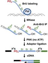
Note: cDNA library preparation and RNA-seq can be outsourced. In Jeandard et al. (2023), Figure S2 shows the key library preparation steps that ensure the selective sequencing of intact transcripts, as briefly summarised below.
Remove caps with RNA 5′-pyrophosphohydrolase.
Ligate the 5′-adapter to 5′-phosphorylated ends.
Ligate the 3′-adapter to 3′-hydroxyl ends.
Perform the first-strand cDNA synthesis using M-MLV reverse transcriptase with a 3′-adapter-annealing primer.
PCR-amplify the resulting cDNA with a high-fidelity DNA polymerase and barcoded TruSeq primers (15 cycles).
Purify cDNA with the AMPure XP kit.
Perform cDNA fragmentation and end repairing and proceed with another round of adapter ligation and PCR amplification.
Pool the cDNA samples equimolarly and perform size-selection on an agarose gel in the range 10–220 nt (excluding the flanking sequences).
Sequence the pool on an Illumina NextSeq 500 instrument (75 nt single-end reads) or similar.
Note: Although the fragmentation step may be expected to destroy the strand-specificity of the protocol, our mapping results (Jeandard et al., 2023) showed that the first 5′-adapter ligation (step G2) largely determines the strandedness of the reads, which permits unambiguous transcript assignment and quantification. Other strategies to enforce the preservation of the strand information can also be implemented (J. Z. Levin et al., 2010; Dar et al., 2016).
Data analysis
The first important information about the success of a CoLoC experiment comes from the analysis of ethidium bromide–stained gels and northern blots. Results of these steps help to evaluate the quality of the RNA samples and make a decision on their suitability for subsequent library preparation (Figure 2). The northern blot signal from the full-size transcript in each sample is analysed by ImageQuant TL or similar densitometry software and normalised by the signal of the spike-in RNA in the same sample. This enables direct measurement of intact transcript levels across the gradient of RNase A concentrations. A well-behaved, informative CoLoC/Mock CoLoC series:
contains at least 9–10 samples with no signs of artefactual degradation (unspecific, irregular RNA degradation is sometimes visible as the appearance of a smear or random bands),
shows a robust signal for the full-size transcript at least in the 0 sample (treated with 0 μg/mL RNase A), which permits reliably measuring the starting level of the RNA of interest,
has a monotonously decreasing pattern for at least some of the probed full-size transcripts, as the RNase concentration increases, indicating that the selected RNase concentration range provides sufficient activity and resolution to plot an informative digestion kinetics.
Note: We strongly recommend probing for a wider variety of transcripts differing in size (50–1,500 nt), structure (loosely structured vs. tightly folded), and localisation, including both bona fide resident RNAs and a few abundant contaminants. If their behaviour corresponds to the expectations of the CoLoC model (gradual disappearance for contaminants; plateauing for residents), it is usually a good indication that such samples can be used for a genome-wide analysis by RNA-seq.
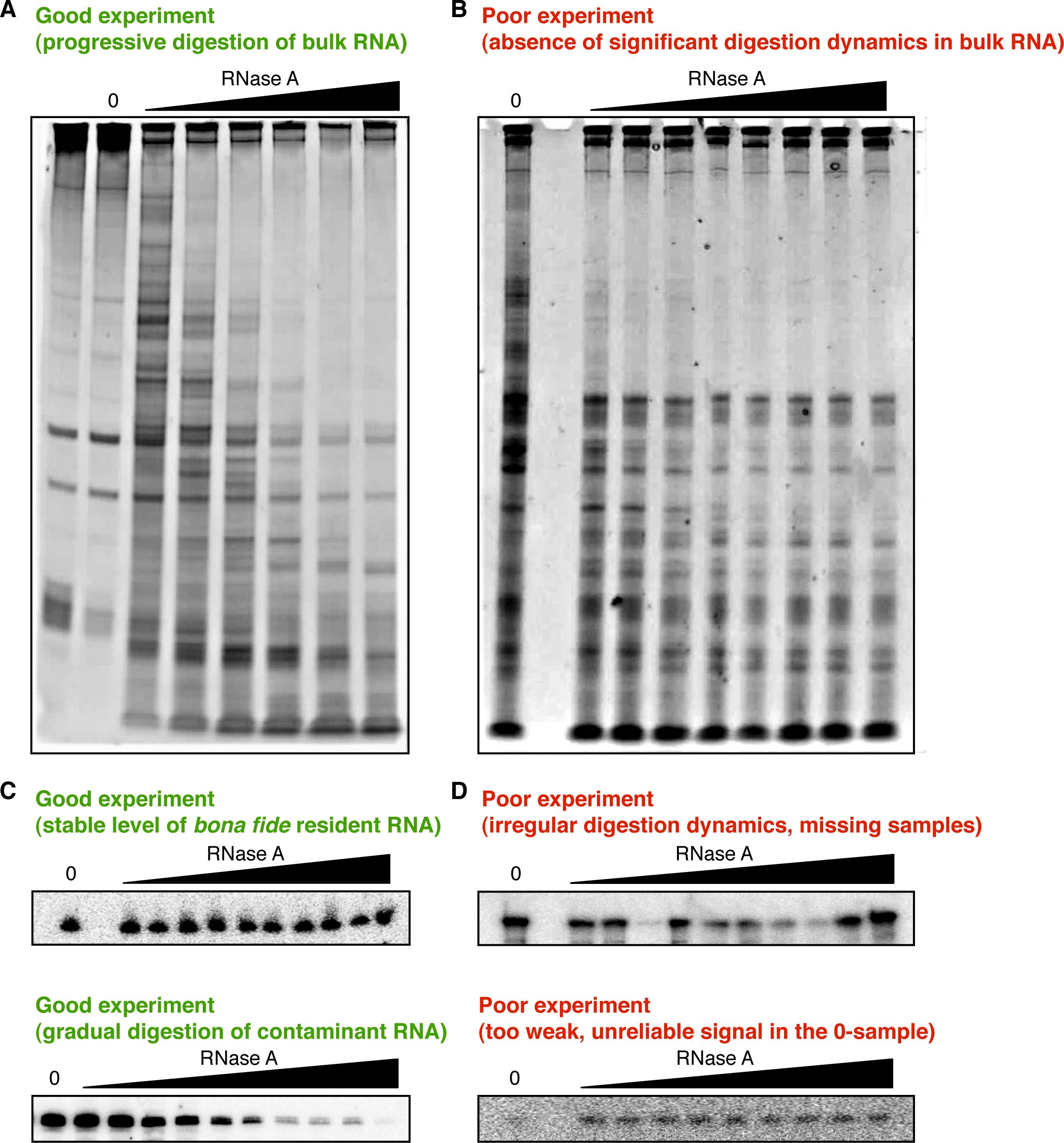
Figure 2. Evaluating the quality of CoLoC samples from ethidium bromide staining and northern blot data. A. This ethidium bromide–stained gel shows an example of a well-behaved series of CoLoC samples. Addition of RNase A provokes gradual bulk RNA degradation, which gets more pronounced as the RNase concentration increases. B. This ethidium bromide–stained gel provides an example of a failed experiment: addition of RNase A has little-to-no effect on bulk RNA; the RNase activity turned out to be insufficient to create meaningful digestion dynamics. C. These northern blots illustrate two successful outcomes of a CoLoC experiment. The upper panel shows an RNase-resistant transcript: its level remains relatively unchanged across the entire gradient of RNase concentrations. The lower panel features an RNase-sensitive RNA, progressively digested with increasing RNase concentrations. D. These northern blots show two examples of less successful experiments. In the upper panel, the transcript level evolves in a fuzzy, indeed random pattern, preventing the fitting of any reasonable kinetics model. In the lower panel, the signal in the 0 sample is too low and cannot be measured with confidence. Therefore, one cannot determine the starting level of this RNA and reliably scale its profile.
Important steps of RNA-seq data treatment are described in Materials and Methods of Jeandard et al. (2023). Briefly, the sequencing reads were pre-processed with cutadapt version 2.8 (Martin, 2011) to trim adapter sequences. Read alignment and gene feature quantification were done with READemption version 0.4.3 (Förstner et al., 2014), using segemehl version 0.2.0-418 (Otto et al., 2014) as the read aligner. All libraries were aligned to the Human genome (Genome Reference Consortium Human Build 38 patch release 13) retrieved from RefSeq (O’Leary et al., 2016). The parameters used for alignment, coverage calculation, and feature quantification can be found in the scripts deposited at Zenodo (https://doi.org/10.5281/zenodo.6389451). Entries for repetitive genes were compounded and their reads were summed up. A cut-off of 30 reads was applied to all 0 samples to ensure reliable initial level measurement. Read counts in each library were normalised by the corresponding number of reads mapping to the spike-in RNA, as described for northern blotting. Read distributions can be visualised in Integrated Genome Browser (v. 9.1.8), Integrative Genomics Viewer, or other similar software. Due to the specifics of the library preparation strategy, the reads typically cluster at the 5′ ends of transcripts. By contrast, if we saw that the overwhelming majority of reads for a certain mRNA- or lncRNA-encoding locus aligned to embedded tRNA-, snRNA-, 7SL-, 5S rRNA-, or mtDNA-like (NUMTs) sequences (usually found in introns), we excluded such genes from the analysis as obvious cross-mapping artefacts.
The quantitative data obtained from northern blots or RNA-seq permits deducing the rate at which RNase A digests the transcript and the relative size of the unreactive pool, protected from the nuclease, using a kinetics model described in detail in Jeandard et al. (2023) in Materials and Methods:
f(A)=(1-P0) e-k'iA+P0 (1)
where f(A) is the relative proportion of the ith transcript remaining after treatment with A μg/mL of RNase A, P0 is the initial protected proportion of the ith transcript (i.e., the part of the ith transcript pool that is unavailable to RNase A, as measured at 0 μg/mL of RNase A), and k’i is the effective digestion rate constant for the ith transcript. Because f(A) is expressed in relative units, the starting transcript level (0 sample) must be normalised to 1, and the remaining samples of the series must be scaled accordingly. To fit the reaction model into the data, we used a customised nonlinear regression function in Origin 2021b, but any other similar software can be used too. Caution: Do not linearize the Equation 1 with the intention to use linear regression instead! Such an approach is misleading as it results in incorrect error modelling, leading to overoptimistic or, on the contrary, strangely poor output statistics. Nonlinear regression software is now widely accessible and quite intuitive. A good general primer in nonlinear regression and associated topics can be found in Motulsky (2010).
Begin by trying to fit the full model (called Model 1 in Jeandard et al., 2023) that has two parameters: the effective digestion rate constant k’ and the initial proportion of RNA protected from digestion P0. It is useful to naturally constrain k’ to be non-negative (k’ ≥ 0) and P0 to be in the range [0,1]. If the software has such an option, it is also recommended to specify as the initial P0 estimate the lowest measured level of the transcript (typically observed in the sample, treated with the highest RNase concentration). This considerably accelerates fitting and increases chances that the fit will converge on a biochemically meaningful combination of parameters reflecting the actual state of the system.
Several regression outcomes are possible (Figure 3). In a successful experiment, the large majority of transcripts yield converging fits, i.e., a certain pre-specified level of the sum of squares of residuals has been reached. This means that k’ and P0 can be reliably estimated for most kinetics (Figure 3A). If this is not the case, the regression software reports a non-converging fit (Figure 3B), which might be either due to low quality of the data (points are too much scattered and do not form any obvious pattern) or because the Model 1 is too complex. In the first case, the data for this specific transcript are, unfortunately, unusable. In the second case, fitting a simpler, nested model may rescue the analysis (see the discussion of this model below):
f(A)=e-k'iA (2)
One should pay attention to—and correctly interpret—the three groups of statistics associated with each fit. The first one is determination coefficient R2. When R2 = 1, the fit is perfect: the model goes through every data point. When R2 = 0, the model is actually a straight horizontal line. (It is also possible in nonlinear regression for R2 to be negative, meaning that the model fits data more poorly than the horizontal line. Such cases are exceptionally rare in CoLoC-seq. See, for example, Figure 3B.) Caution: It is a common misconception to conclude that low R2 means poor model fit! The quality of fitting can only be evaluated by looking at the residuals, and if the regression software says that the fit converged, it means that the residuals are small enough. Therefore, the fit can actually converge on a horizontal line (R2 = 0) as the best model fitting the data (Figure 3C). This case is typical for resident or RNase-resistant transcripts: their level is unaffected by increasing RNase concentration and, within the limits of the random error, remains constant (i.e., the graph is a horizontal line).
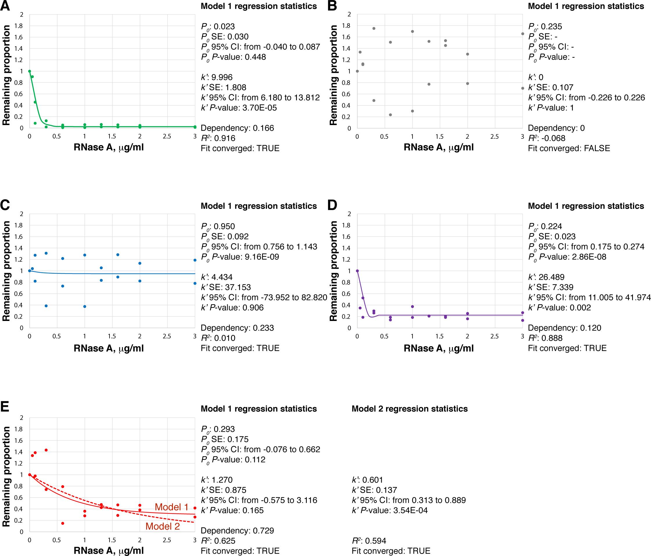
Figure 3. Real-life examples of CoLoC-seq data and their analysis by nonlinear regression, performed in Origin 2021b. A. Well-behaved series showing a typical RNase-sensitive transcript. P0 is nearly 0 and insignificant; k’ is high and significant. Dependency is low, indicating that P0 and k’ have been estimated independently from each other; R2 is high; the fit converged. B. Example of a failed series: the data points are too much scattered; as a result, the fit did not converge. C. This successful series shows a typical behaviour of a transcript protected from RNase: with the exception of a couple of outliers, the data points align close to the horizontal line with P0 ≈ 1. k’ is insignificant, indicating that no appreciable degradation of this transcript occurred. R2 is nearly 0 (i.e., horizontal line), but the fit converged well. D. This well-behaved series shows a transcript that is partially protected from RNase. Both P0 and k’ are significantly non-zero, indicating that the population of this RNA was digested to some extent and plateaued at the level of 0.224 (i.e., 22.4% of this transcript pool is estimated to be protected from RNase). E. Fitting the Model 1 (solid line) into this series resulted in highly entangled and unreliable P0 and k’ estimates (dependency 0.729), suggesting that the two variables are significantly collinear, and the model is unnecessarily complex. Fitting the simpler Model 2 (which does not have the P0 parameter; dashed line) permitted a more reliable estimation of k’. Note that the two models yield almost indistinguishable fits; however, the Model 2 is more parsimonious, which explains its success in estimating k’. See Jeandard et al. (2023), Table S2 for further examples.The second group of statistics concerns the best-fit values of the parameters and the associated uncertainty measures. The parameter of primary interest is P0. When P0 ≈ 0, there is no sizable protected pool for the ith RNA, meaning that it fully participates in the reaction (Figure 3A). Therefore, under the CoLoC-seq setup, such an RNA is a regular, degradable contaminant. We operationally consider that all transcripts with P0 < 0.1 are potential contaminants (see Figure 3C in Jeandard et al., 2023). By contrast, when P0 is considerably larger (P0 > 0.1, Figure 3D), a significant proportion (> 10%) of the ith RNA does not participate in the reaction, i.e., it is somehow protected from RNase A (with P0 = 1 meaning that 100% of the transcript is protected). How exactly protected depends on the results of CoLoC-seq vs. Mock CoLoC-seq experiments. If the transcript shows high P0 in CoLoC-seq but not in Mock CoLoC-seq, where the organellar membranes have been dissolved, one can consider this as evidence that a pool of this transcript genuinely resides inside the organelle, and its protection was due to the membranes. By contrast, if both CoLoC-seq and Mock CoLoC-seq return high P0 values, this means that the transcript in question is intrinsically resistant to RNase A, and its protection has nothing to do with the organellar membranes. As discussed on several examples in Jeandard et al. (2023), such transcripts are most likely false positives.
The best-fit value of k’ may also be of interest. For example, when k’ ≈ 0 (Figure 3C), it means that the transcript in question practically does not undergo degradation, and the initial Model 1 degenerates to the simplistic Model 3, i.e., a horizontal line:
f(A) = 1 (3)
The best-fit values should be interpreted along with the accompanying uncertainty statistics. These are often returned as standard errors (SE) or, more conveniently, confidence intervals (CI). Narrow SE or CI mean that the corresponding parameters (P0 or k’) are estimated with precision. Importantly, when the CI for P0 includes 0, it means that P0 is not significantly different from 0, i.e., there is no strong evidence for the existence of a protected pool for this transcript. When the CI for k’ includes 0, it means that the digestion rate is insignificant, that there is no strong evidence that RNase A actually cleaves this RNA (i.e., the transcript is protected). Under the CoLoC-seq setup, regular, degradable contaminants typically show low P0 values, with CIs including 0, and relatively high k’ values, with CIs far from 0 (Figure 3A). By contrast, protected transcripts feature relatively high P0 values, with CIs far from 0; their k’ values can vary, depending on the proportion of the ith RNA available for degradation (Figure 3C and 3D).
The best-fit values of parameters are often accompanied by P-values conveying similar information (the null hypothesis being that the true value of the parameter is 0). A low P-value suggests that the parameter is likely non-zero. Under the CoLoC-seq setup, degradable contaminants often show high P-values for P0 and low P-values for k’ (Figure 3A). By contrast, resident transcripts should normally have low P-values for P0 (Figure 3C, D). A high P-value (and a CI including 0) means that the corresponding parameter is not useful, i.e., the complete Model 1 can be simplified to the nested Model 2 (simple pseudo-first order decay) or the Model 3 (no decay).
The last part of regression statistics, which is very important to take in consideration, is the dependency between parameters. Dependency is the degree of entanglement between the estimated parameters. In some situations, especially where the RNase-mediated digestion is very slow or even inexistant, P0 and k’ become significantly collinear, and the regression software struggles to fit them separately since small changes in either of them yield nearly equivalent results (Figure 3E). In Jeandard et al. (2023), we arbitrarily used the dependency cutoff of 0.3, above which we considered P0 and k’ to be too much entangled to speak about their independent fitting. This threshold can be reviewed when applying CoLoC-seq to other systems. Just like the uncertainty parameters discussed above, high dependency means that the Model 1 is unnecessarily complex, and one of the parameters must be dropped.
Since the Model 3 is always implicitly tested by the regression software (see the discussion of R2 above), one can only omit P0 from the model, thus yielding the Model 2. Therefore, if by using the complete Model 1 the fit does not converge, or one of the estimated parameters is not significant, or there is strong interdependency between the parameters, one should try to fit the simpler Model 2 into the data. This usually helps to rescue for analysis the profiles of the majority of remaining transcripts and especially those with a high level of protection from RNase A (i.e., the transcripts of highest interest for CoLoC-seq). The Model 2 has only one explicit parameter, k’. Interpretation of the results of this regression follows the same reasoning as for the Model 1, with high significant k’ corresponding to degradable transcripts, while low insignificant k’ means protection (one can assign such transcripts a nominal P0 of 1). The decision making is summarized in Table 1.
We recommend using at least two biological replicates for CoLoC-seq and Mock CoLoC-seq. If the replicates are very similar to each other, it makes sense to combine them for model fitting and thereby increase the power and precision of the regression, while preserving the information about biological variability of the original samples. The similarity of the replicates can be evaluated at several levels: (i) by plotting read counts for the same transcript from different replicates at the same RNase concentration, or (ii) by fitting the Model 1 separately for each replicate and plotting together the P0 values from different replicates (see for an example Figure S6 in Jeandard et al., 2023). The latter test is more stringent.
Validation of protocol
We evaluated the feasibility and performance of CoLoC-seq on the well-studied mitochondrial transcriptome of human embryonic kidney 293 (HEK293) cells (Jeandard et al., 2023). To this end, two biological replicate series of CoLoC-seq and Mock CoLoC-seq samples were analysed by northern blotting and RNA-seq. The replicates were very similar to each other and yielded highly correlated P0 values (Figure S6 in Jeandard et al., 2023), confirming the intra-method reproducibility. The RNA levels and the fitted P0 values obtained from RNA-seq and northern blotting measurements also showed excellent agreement (Figure 2 and Figure S5 in Jeandard et al., 2023), indicating that CoLoC-seq correctly captures quantitative information about the kinetic behaviour of analysed transcripts. No significant bias at the level of transcript abundance, sequence, or structure was observed (Figure S7 in Jeandard et al., 2023). However, due to limitations of the standard RNA-seq protocol, the representation of tRNAs in the RNA-seq libraries was generally biased against extensively modified species (Figure S8 in Jeandard et al., 2023).
The behaviour of transcripts in the CoLoC-seq and Mock CoLoC-seq setups was significantly different (Figures 3 and 4 and Figure S6 in Jeandard et al., 2023), indicating that the mitochondrial membranes do provide shelter for a subset of RNA molecules. As expected, the mitochondrial DNA-encoded mitochondrial RNAs were mostly resistant to RNase A in the CoLoC-seq setup but rapidly degraded in Mock CoLoC-seq, confirming that they are genuinely present inside the organelles. By contrast, the vast majority of nuclear DNA-encoded transcripts, such as the abundant 5.8S rRNA and U6 snRNA, were rapidly degraded in both cases, confirming that they are surface-attached degradable contaminants (Figures 2–4 in Jeandard et al., 2023). Of note, a few short, highly structured, and protein-bound noncoding transcripts, such as 5S rRNA and the RNA components of RNases P and MRP, plateaued at an intermediate level in both the CoLoC-seq and the Mock CoLoC-seq experiments. This indicates that they remained, to a large extent, resistant to RNase degradation even when the mitochondrial membranes had been dissolved and may, therefore, represent recalcitrant contaminants. We also identified a few RNA Pol III transcripts, such as Y RNAs, SNAR-A, and tRNAs, as likely partially mitochondria-localised (Figure 4 and Figure S8 in Jeandard et al., 2023), which was further corroborated by biochemical and smFISH assays (Figure 5 in Jeandard et al., 2023).
Table 1. Decision making criteria to interpret CoLoC-seq regression data
| Model 1 (complete) | ||||||||||||
| CoLoC-seq | Mock CoLoC-seq | Interpretation | ||||||||||
| P0 | P0 CI includes 0? | P0 P-value | k’ | k’ CI includes 0? | k’P-value | P0 | P0 CI includes 0? | P0 P-value | k’ | k’ CI includes 0? | k’P-value | |
| ≈0 | Usually yes* | Usually high* | High | No | Low | ≈0 | Usually yes* | Usually high* | High | No | Low | Degradable contaminant |
| Far from 0 but < 1 | No | Low | High | No | Low | ≈0 | Usually yes* | Usually high* | High | No | Low | Partially resident inside the organelle |
| ≈1 | No | Low | ≈0 | Yes | High | ≈0 | Usually yes* | Usually | High | No | Low | Fully resident inside the organelle |
| Far from 0 but < 1 | No | Low | High | No | Low | Far from 0 but < 1 | No | Low | High | No | Low | Partially RNase-resistant transcript |
| ≈1 | No | Low | ≈0 | Yes | High | ≈1 | No | Low | ≈0 | Yes | High | RNase-resistant transcript |
| Model 2 (pseudo-first order decay) | ||||||||||||
| k’ | k’ CI includes 0? | k’P-value | k’ | k’ CI includes 0? | k’P-value | Interpretation | ||||||
| High | No | Low | High | No | Low | Degradable contaminant | ||||||
| ≈0 | Yes | High | High | No | Low | Fully resident inside the organelle | ||||||
| ≈0 | Yes | High | ≈0 | Yes | High | RNase-resistant transcript | ||||||
*The CI width and the P-value largely depend on the sample size, and at a high enough n it is quite common to obtain statistically significant results even for very small P0 values (close to 0). In such situations, one should rely more on the absolute value of P0: if it is very small, it is reasonable to consider such a transcript as fully degradable (i.e., contaminant, under the CoLoC-seq setup), even if the uncertainty measures seem to be "highly significant". In Jeandard et al. (2023), given the limited precision of RNA level measurements by northern blotting and by RNA-seq, we arbitrarily chose the P0 cut-off of 0.1. This means that at least 10% of the transcript needs to be excluded from the reaction to speak about a significant level of protection. See also the discussion of unusually small yet significant k’ values in Table S2 in Jeandard et al. (2023).
Since the mitochondrial transcriptome of human cells has become a popular benchmark for subcellular transcriptomics (Mercer et al., 2011; Kaewsapsak et al., 2017; Fazal et al., 2019; P. Wang et al., 2019; Zhou et al., 2019), we could directly compare the CoLoC-seq performance with that of other genome-wide methods (especially, the most robust proximity labelling techniques). We found that CoLoC-seq performed equally well on long transcripts (rRNAs, mRNAs, lncRNAs) and significantly outperformed alternative methods on shorter transcripts (tRNAs, snRNAs, snoRNAs, scaRNAs etc.), which are generally poorly covered by proximity labelling approaches.
General notes and troubleshooting
General notes
One should take into account two important points when choosing the RNase for CoLoC-seq experiments: (i) it should behave as a kinetically perfect enzyme, i.e., its catalysis must be limited only by diffusion (Park and Raines, 2003) and (ii) it should produce 5′-hydroxyl and 2′- or 3′-phosphate termini. The first property enables a straightforward use of the CoLoC-seq kinetics model, which implies that diverse transcripts in the sample are cleaved independently, without significant RNase-sequestration effects; therefore, the RNase concentration can be considered constant, and the entire reaction becomes pseudo-first order. The second property permits selective sequencing of intact transcripts (as required by the CoLoC-seq model, which only looks at remaining intact RNA; see Eq. 1): a single cleavage by such an RNase generates a terminus incompatible with standard adaptor ligation (see the section G. Library preparation & RNA-seq). (The caveat here is that one cannot study transcripts with natural 5′-OH or 2′- or 3′-phosphorylated ends by RNA-seq. However, they remain analysable by northern blotting.) Other highly active RNases generating 5′-hydroxyl and 2′- or 3′-phosphate termini (micrococcal nuclease, RNase I, RNase T1) could in principle be used too. However, we and others found them to be overall less well performing and more idiosyncratic than RNase A [Yang, 2011; Aryani and Denecke, 2015; Jeandard et al., 2023 (Figure S1)].
The exact RNase concentrations used in CoLoC-seq depend on the specific activity of the enzyme batch and the nature of the studied biological material. They should be adjusted individually for every new application. It is essential that the selected concentration range enables the observation of gradual digestion dynamics of contaminant transcripts without compromising the quality of the final RNA samples (Figure 2A, 2B). One should strive to get particularly high resolution at low RNase concentrations, where a small change in RNase typically results in a big change in the remaining transcript level (Figure 3A, 3D). This facilitates k’ fitting and thereby increases the precision of the P0 estimate.
CoLoC-seq can be applied to nearly any membrane-bounded organelles (see, for example, the previously published isolation protocols for chloroplasts and apicoplasts: Kunst, 1998; Botté et al., 2018) and other entities known or suspected to contain RNA (viruses, endosymbiotic organisms, extracellular vesicles). Since extracellular RNA can be packaged in and protected by membranous vesicles, such as exosomes, but also by free RNPs, researchers that wish to adapt CoLoC-seq to such systems may need to incorporate a proteinase K pre-treatment step to expose RNP-embedded contaminants and enable their subsequent digestion by RNase (Arroyo et al., 2011; Hill et al., 2013; Mateescu et al., 2017; Jeppesen et al., 2019; Murillo et al., 2019; Gruner and McManus, 2021).
Finally, due to intrinsically low susceptibility of miRNAs to RNase-mediated degradation (especially when they are associated with proteins, as it is typically the case), we discourage using CoLoC-seq (or indeed other RNase-based approaches) to infer their localisation topology (Arroyo et al., 2011; Aryani and Denecke, 2015).
Troubleshooting (Table 2)
Table 2. Troubleshooting
| Problem | Possible cause | Solutions |
| Presence of unspecific RNA degradation in samples (smear, additional random bands) | • RNase contamination in water. • RNase contamination from air. • RNase contamination of pipette filters. | • Prepare all solutions on RNase-free water. • Work in a dedicated RNase-free environment. • Change pipette filters. |
| Low RNA yield | • Insufficient starting material. • Poor organelle yield. | • Increase the amount of the starting material. • Try an alternative organelle isolation protocol with a higher yield. |
| Uneven pattern across samples upon ethidium bromide staining or northern blotting (e.g., Figure 2D) | • Organelle pellet was unevenly or insufficiently resuspended between samples. • Non-uniform RNA isolation. • Insufficiently solubilised RNA pellets. | • Resuspend the organelle pellet carefully but thoroughly before splitting it into the sample series. Use a narrower pipette tip, if required. • Make sure that the aqueous phase is taken up uniformly between samples. Always process samples in the same order to make their treatment maximally identical. • If you suspect that the RNA pellet is not fully dissolved (often due to protein contamination), re-extract all samples with TRIzol. |
| Poor digestion dynamics showing either insignificant (e.g., Figure 2B) or, on the contrary, too rapid RNA degradation across samples | • Too low/high RNase activity or concentration range. • Suboptimal reaction conditions. | • Increase/decrease the amount of RNase. • Change the enzyme batch. • Increase/decrease reaction temperature (between 0 and 37 °C). • Increase/decrease reaction time (1–15 min). • Try to adjust the salt concentration, specific divalent cations, or pH, based on known RNase preferences. • We recommend, before attempting the complete CoLoC-seq experiment, to perform test digestions in total cell or organelle lysates (as described in part D of the protocol), using a variety of enzymes and reaction conditions (see Figure S1 in Jeandard et al., 2023). |
| In the CoLoC-seq setup, bona fide resident transcripts are degraded as if they were contaminants | • Too harsh isolation protocol compromised the integrity of the organelles. | • Use a milder cell disruption and/or organelle isolation protocol. |
| In the CoLoC-seq setup, all RNAs look at least partially protected | • Cells were not sufficiently disrupted. • Cell debris contaminated the organelle prep. | • Use additional/stronger disruption and check the material under a light microscope. • Add an additional low-speed centrifugation step to further remove cell debris. • Take up the supernatant after the low-speed centrifugation more cleanly, discarding the lower part of the supernatant together with the debris pellet. |
| Poor RNA yield in the Mock CoLoC-seq setup | • Insufficient lysis of the organelles. | • Use a stronger/more concentrated non-ionic detergent. • Apply extra mechanical force (Dounce homogeniser, syringe, sonication; but beware of RNA shearing!). |
Acknowledgments
This work was supported by the University of Strasbourg through the IdEx Unistra [ANR-10-IDEX-0002], the SFRI-STRAT_US project [ANR 20-SFRI-0012], EUR IMCBio [ANR17-EURE-0023], and IdEx – Attractivité [ANR-10-IDEX-0002-02 to Al.S.], and by the Centre National de la Recherche Scientifique (CNRS). The CoLoC-seq method was first published in Jeandard et al. (2023).
Competing interests
There are no conflicts of interest or competing interests.
References
- Arroyo, J. D., Chevillet, J. R., Kroh, E. M., Ruf, I. K., Pritchard, C. C., Gibson, D. F., Mitchell, P. S., Bennett, C. F., Pogosova-Agadjanyan, E. L., Stirewalt, D. L., et al. (2011). Argonaute2 complexes carry a population of circulating microRNAs independent of vesicles in human plasma. Proc. Natl. Acad. Sci. U. S. A. 108(12): 5003–5008.
- Aryani, A. and Denecke, B. (2015). In vitro application of ribonucleases: comparison of the effects on mRNA and miRNA stability. BMC Res. Notes 8(1): e1186/s13104-015-1114-z.
- Botté, C. Y., McFadden, G. I. and Yamaryo-Botté, Y. (2018). Isolating the Plasmodium falciparum Apicoplast Using Magnetic Beads. In: Maréchal, E. (Ed.). Plastids (pp. 205–212). Methods in Molecular Biology. Humana Press, New York.
- Bresnahan, W. A. and Shenk, T. (2000). A Subset of Viral Transcripts Packaged Within Human Cytomegalovirus Particles. Science 288(5475): 2373–2376.
- Dar, D., Shamir, M., Mellin, J. R., Koutero, M., Stern-Ginossar, N., Cossart, P. and Sorek, R. (2016). Term-seq reveals abundant ribo-regulation of antibiotics resistance in bacteria. Science 352(6282): eaad9822.
- Engel, K. L., Lo, H. Y., Goering, R., Li, Y., Spitale, R. C. and Taliaferro, J. M. (2021). Analysis of subcellular transcriptomes by RNA proximity labeling with Halo-seq. Nucleic Acids Res. 50(4): e24–e24.
- Fazal, F. M., Han, S., Parker, K. R., Kaewsapsak, P., Xu, J., Boettiger, A. N., Chang, H. Y. and Ting, A. Y. (2019). Atlas of Subcellular RNA Localization Revealed by APEX-Seq. Cell 178(2): 473–490.e26.
- Förstner, K. U., Vogel, J. and Sharma, C. M. (2014). READemption--a tool for the computational analysis of deep-sequencing-based transcriptome data. Bioinformatics 30(23): 3421–3423.
- Geiger, J. and Dalgaard, L. T. (2017). Interplay of mitochondrial metabolism and microRNAs. Cell. Mol. Life Sci. 74(4): 631–646.
- Gruner, H. N. and McManus, M. T. (2021). Examining the evidence for extracellular RNA function in mammals. Nat. Rev. Genet. 22(7): 448–458.
- Hill, A. F., Pegtel, D. M., Lambertz, U., Leonardi, T., O’Driscoll, L., Pluchino, S., Ter-Ovanesyan, D. and Nolte-‘t Hoen, E. N. (2013). ISEV position paper: extracellular vesicle RNA analysis and bioinformatics. J. Extracell. Vesicles 2(1): 22859.
- Höltke, H. J., Sagner, G., Kessler, C. and Schmitz, G. (1992). Sensitive chemiluminescent detection of digoxigenin-labeled nucleic acids: a fast and simple protocol and its applications. Biotechniques 12(1): 104–113.
- Jeandard, D., Smirnova, A., Fasemore, A. M., Coudray, L., Entelis, N., Förstner, K. U., Tarassov, I. and Smirnov, A. (2023). CoLoC-seq probes the global topology of organelle transcriptomes. Nucleic Acids Res. 51(3): e16–e16.
- Jeandard, D., Smirnova, A., Tarassov, I., Barrey, E., Smirnov, A. and Entelis, N. (2019). Import of Non-Coding RNAs into Human Mitochondria: A Critical Review and Emerging Approaches. Cells 8(3): 286.
- Jeppesen, D. K., Fenix, A. M., Franklin, J. L., Higginbotham, J. N., Zhang, Q., Zimmerman, L. J., Liebler, D. C., Ping, J., Liu, Q., Evans, R., et al. (2019). Reassessment of Exosome Composition. Cell 177(2): 428–445.e18.
- Kaewsapsak, P., Shechner, D. M., Mallard, W., Rinn, J. L. and Ting, A. Y. (2017). Live-cell mapping of organelle-associated RNAs via proximity biotinylation combined with protein-RNA crosslinking. eLife 6: e29224.
- Kunst, L. (1998). Preparation of Physiologically Active Chloroplasts from Arabidopsis. In: Martinez-Zapater, J. M. and Salinas, J. (Eds.). Arabidopsis Protocols (pp. 43–48). Methods in Molecular BiologyTM. Humana Press.
- Lécrivain, A. L. and Beckmann, B. M. (2020). Bacterial RNA in extracellular vesicles: A new regulator of host-pathogen interactions? Biochim. Biophys. Acta Gene Regul. Mech. 1863(7): 194519.
- Levin, J. Z., Yassour, M., Adiconis, X., Nusbaum, C., Thompson, D. A., Friedman, N., Gnirke, A. and Regev, A. (2010). Comprehensive comparative analysis of strand-specific RNA sequencing methods. Nat. Methods 7(9): 709–715.
- Levin, L., Blumberg, A., Barshad, G. and Mishmar, D. (2014). Mito-nuclear co-evolution: the positive and negative sides of functional ancient mutations. Front. Genet. 5: e00448.
- Martin, M. (2011). Cutadapt removes adapter sequences from high-throughput sequencing reads. EMBnet. J. 17(1): 10.
- Mateescu, B., Kowal, E. J. K., van Balkom, B. W. M., Bartel, S., Bhattacharyya, S. N., Buzás, E. I., Buck, A. H., de Candia, P., Chow, F. W. N., Das, S., et al. (2017). Obstacles and opportunities in the functional analysis of extracellular vesicle RNA – an ISEV position paper. J. Extracell. Vesicles 6(1): 1286095.
- Medina-Munoz, H. C., Lapointe, C. P., Porter, D. F. and Wickens, M. (2020). Records of RNA locations in living yeast revealed through covalent marks. Proc. Natl. Acad. Sci. U. S. A. 117(38): 23539–23547.
- Mercer, T. R., Neph, S., Dinger, M. E., Crawford, J., Smith, M. A., Shearwood, A. M., Haugen, E., Bracken, C. P., Rackham, O., Stamatoyannopoulos, J. A., et al. (2011). The Human Mitochondrial Transcriptome. Cell 146(4): 645–658.
- Miller, B. R., Wei, T., Fields, C. J., Sheng, P. and Xie, M. (2018). Near-infrared fluorescent northern blot. RNA 24(12): 1871–1877.
- Motulsky, H. (2010). Intuitive biostatistics: a nonmathematical guide to statistical thinking (Completely rev. 2nd ed). New York: Oxford University Press.
- Murillo, O. D., Thistlethwaite, W., Rozowsky, J., Subramanian, S. L., Lucero, R., Shah, N., Jackson, A. R., Srinivasan, S., Chung, A., Laurent, C. D., et al. (2019). exRNA Atlas Analysis Reveals Distinct Extracellular RNA Cargo Types and Their Carriers Present across Human Biofluids. Cell 177(2): 463–477.e15.
- O’Leary, N. A., Wright, M. W., Brister, J. R., Ciufo, S., Haddad, D., McVeigh, R., Rajput, B., Robbertse, B., Smith-White, B., Ako-Adjei, D., et al. (2016). Reference sequence (RefSeq) database at NCBI: current status, taxonomic expansion, and functional annotation. Nucleic Acids Res. 44: D733–D745.
- Otto, C., Stadler, P. F. and Hoffmann, S. (2014). Lacking alignments? The next-generation sequencing mapper segemehl revisited. Bioinformatics 30(13): 1837–1843.
- Park, C. and Raines, R. T. (2003). Catalysis by Ribonuclease A Is Limited by the Rate of Substrate Association. Biochemistry 42(12): 3509–3518.
- Quirós, P. M., Mottis, A. and Auwerx, J. (2016). Mitonuclear communication in homeostasis and stress. Nat. Rev. Mol. Cell Biol. 17(4): 213–226.
- Routh, A., Domitrovic, T. and Johnson, J. E. (2012). Host RNAs, including transposons, are encapsidated by a eukaryotic single-stranded RNA virus. Proc. Natl. Acad. Sci. U. S. A. 109(6): 1907–1912.
- Schneider, A. (2011). Mitochondrial tRNA Import and Its Consequences for Mitochondrial Translation. Annu. Rev. Biochem. 80(1): 1033–1053.
- Sieber, F., Duchêne, A.-M. and Maréchal-Drouard, L. (2011). Mitochondrial RNA import: from diversity of natural mechanisms to potential applications. Int. Rev. Cell Mol. Biol. 287: 145–190.
- Wang, K., Zhang, S., Weber, J., Baxter, D. and Galas, D. J. (2010). Export of microRNAs and microRNA-protective protein by mammalian cells. Nucleic Acids Res. 38(20): 7248–7259.
- Wang, P., Tang, W., Li, Z., Zou, Z., Zhou, Y., Li, R., Xiong, T., Wang, J. and Zou, P. (2019). Mapping spatial transcriptome with light-activated proximity-dependent RNA labeling. Nat. Chem. Biol. 15(11): 1110–1119.
- Woodson, J. D. and Chory, J. (2008). Coordination of gene expression between organellar and nuclear genomes. Nat. Rev. Genet. 9(5): 383–395.
- Yang, W. (2011). Nucleases: diversity of structure, function and mechanism. Q. Rev. Biophys. 44(1): 1–93.
- Zhou, Y., Wang, G., Wang, P., Li, Z., Yue, T., Wang, J. and Zou, P. (2019). Expanding APEX2 Substrates for Proximity‐Dependent Labeling of Nucleic Acids and Proteins in Living Cells. Angew. Chem. Int. Ed. 58(34): 11763–11767.
Supplementary information
- Scripts used for read alignment, coverage calculation, and feature quantification of human mitochondrial CoLoC-seq data can be found on Zenodo (https://doi.org/10.5281/zenodo.6389451).
- The CoLoC-seq and Mock-CoLoC-seq sequencing data published in Jeandard et al. (2023) were deposited in NCBI Gene Expression Omnibus (GEO) under accession number GSE183167 (https://www.ncbi.nlm.nih.gov/geo/query/acc.cgi?acc=GSE183167).
Article Information
Publication history
Published: Sep 20, 2023
Copyright
© 2023 The Author(s); This is an open access article under the CC BY-NC license (https://creativecommons.org/licenses/by-nc/4.0/).
How to cite
Smirnova, A., Jeandard, D. and Smirnov, A. (2023). Controlled Level of Contamination Coupled to Deep Sequencing (CoLoC-seq) Probes the Global Localisation Topology of Organelle Transcriptomes. Bio-protocol 13(18): e4820. DOI: 10.21769/BioProtoc.4820.
Category
Molecular Biology > RNA > RNA localisation
Molecular Biology > RNA > RNA sequencing
Systems Biology > Transcriptomics > RNA-seq
Do you have any questions about this protocol?
Post your question to gather feedback from the community. We will also invite the authors of this article to respond.
![]() Tips for asking effective questions
Tips for asking effective questions
+ Description
Write a detailed description. Include all information that will help others answer your question including experimental processes, conditions, and relevant images.